Garner DM1*, Bernardo AFB2 and Vanderlei LCM2
1Cardiorespiratory Research Group, Department of Biological and Medical Sciences, Faculty of Health and Life Sciences, Oxford Brookes University, Headington Campus, Gipsy Lane, United Kingdom
2Department of Physiotherapy, Sao Paulo State University, UNESP, Sao Paulo, Brazil
*Correspondence: David M Garner, Cardiorespiratory Research Group, Department of Biological and Medical Sciences, Faculty of Health and Life Sciences, Oxford Brookes University, Headington Campus, Gipsy Lane, United Kingdom
Received on 12 January 2021; Accepted on 19 February 2021; Published on 04 March 2021
Copyright © 2021 Garner DM, et al. This is an open access article and is distributed under the Creative Commons Attribution License, which permits unrestricted use, distribution, and reproduction in any medium, provided the original work is properly cited.
Abstract
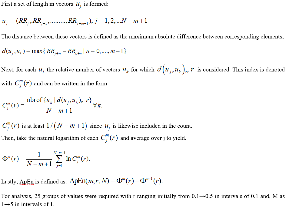
Introduction: Approximate entropy (ApEn) is a widely imposed metric to evaluate a chaotic response and irregularities of RR-intervals from an electrocardiogram. Yet, the technique is problematic due to the accurate choice of the tolerance (r) and embedding dimension (M). We prescribed the metric to evaluate these responses in subjects exhibiting symptoms of chronic obstructive pulmonary disease (COPD) and we strived to overcome this disadvantage by applying different groupings to detect the optimal.
Methods: We examined 38 subjects split equally: COPD and control. To evaluate autonomic modulation the heart rate was measured beat-by-beat for 30 min in a supine position without any physical, sensory, or pharmacological stimuli. In the time-series obtained the ApEn was then applied with set values for tolerance, r and embedding dimension, M. Then, the differences between the two groups and their effect size by two measures (Cohen’s ds and Hedges’s gs) were computed.
Results: The highest value of statistical significance accomplished for any effect size statistical combinations undertaken was -1.13 for Cohen’s ds, and -1.10 for Hedges’s gs with embedding dimension, M = 2 and tolerance, r = 0.1.
Conclusion: ApEn was capable of optimally identifying the decrease in chaotic response in COPD. The optimal combination of r and M for this were 0.1 and 2, respectively. Despite this, ApEn is a relatively unpredictable mathematical marker and the use of other techniques to evaluate a healthy or pathological condition is encouraged.
Keywords
COPD, approximate entropy, HRV, tolerance, embedding dimension, effect sizes
Abbreviations
ApEn: approximate entropy; COPD: chronic obstructive pulmonary disease; HRV: heart rate variability; ANS: autonomic nervous system; DM1: type 1 diabetes mellitus
Introduction
RR-interval rhythm, obtained via an electrocardiographic trace, can deviate in an uneven and often chaotic manner [1–4]. Computational signal processing of physiological data has stimulated academics to investigate this area of research [5, 6]. Heart rate variability (HRV) is an easy, dependable and relatively cheap technique to monitor the autonomic nervous system (ANS) and, a useful technique for judging healthy and pathological states [7–9]. Alternative methods to monitor the ANS are either insensitive for example, sympathetic skin response [10, 11] or too complicated and overpriced such as, quantitative pupillography [12]. Chaotic performances in biological and medical dynamical systems may specify normal physiological status but, loss of chaotic tendencies could be an abnormal and pathological marker [13].
HRV can be evaluated by means of approximate entropy (ApEn) [14]. The benefits of ApEn include low computational processor demand and it can adapt to short time-series (RR < 50). Accordingly, it could be a candidate metric to be enforced online in clinics or critical care units, where processing speed is imperative. Additionally, it can decipher statistics accurately even in the presence of considerable signal noise.
Regrettably, it has a key disadvantage that it is excessively dependent on parameter choices for its tolerance, r and embedding dimension, M. So, ApEn results are unpredictable and difficult to interpret, when compared to the other techniques, such as the chaotic global procedures [2, 13, 15, 16].
In this context, we enforced different combinations for r and M in subjects exhibiting chronic obstructive pulmonary disease (COPD) [17–19] symptoms and those without with the objective of locating the most statistically significant ones to categorize the two groups and develop an application of ApEn which can separate their datasets. This is important to offer a useful clinical and analytical tool for clinicians and other health professionals to make necessary decisions.
Methods: Patient Selection and Assessment
A total of 38 subjects were studied. 19 exhibited the clinical symptoms of COPD and 19 were considered normal and designated controls in the study. Data was logged with a controlled laboratory temperature between 21°C and 24°C, and humidity between 50% and 60%. Subjects were instructed to avoid consumption of alcoholic beverages and caffeinated drinks or heavy foodstuffs for 24 h prior to the assessments. The experimental procedures were completed between 8:00 am and 11:00 am to minimalize circadian rhythm interferences. All actions needed for the data collection were described to the individuals, and the subjects were instructed to continue at rest and to avoid speaking throughout the experiment [20].
Following the preliminary evaluation, the heart monitor strap was placed on the subject’s thorax at the level of the distal third of the sternum. The HR equipment (Polar S810i monitor, Polar Electro OY, Kempele, Finland) was attached to the wrist [9, 21]. This apparatus had been formerly validated for HRV analysis. The subjects were supinely positioned and stationary with 30 min of spontaneous breathing.
To authenticate the COPD diagnosis, the forced vital capacity test was performed [22] pre-bronchodilator to post-bronchodilator [23, 24] via a portable spirometer (MIR, Spirobank version 3.6, Italy) linked to a computer using WinspiroPRO 1.1.6 software. The forced expiratory volume in one second (FEV1) should be ≥80% of the projected normal values with a FEV1/FVC (forced vital capacity) namely < 70%, which is considered the bronchial obstruction threshold [23].
HRV was logged throughout the monitoring process with a sampling rate of 1 kHz. Precisely, 1000 RR intervals were selected for analysis after digital and manual filtering for the elimination of untimely ectopic beats and artefacts. Only series with > 95% sinus rhythm were considered in the final study.
Mathematical Assessment
Entropy based approaches are frequently required for physiological data and signal analysis [25–28]. ApEn [26, 28–30], is a metric that assesses the level of regularity and unpredictability of time-series fluctuations. ApEn is the logarithmic ratio of component-wise matching sequences from the signal length, N. Further constraints include r for tolerance and M for the embedding dimension. A value of zero for ApEn would indicate a totally predictable series. ApEn rises with increasing chaotic response and irregularities. ApEn is described algebraically in the Kubios HRV® analysis manual [31].
Effect sizes
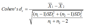
We assessed two effect sizes [32–34] to consider the datasets significances. We excluded any assessments of normality [35–37] usually followed by the application of the one-way analysis of variance [38] (ANOVA1), or Kruskal-Wallis tests [39]. These two statistical approaches are unable to discriminate sufficiently between the small changes in significance that are apparent here.
Cohen’s ds is the principal subcategory. It refers to the standardized mean difference between two groups of independent observations for a suitable sample [40]. It is formulated on the sample means and gives a biased approximation of the population effect size, with samples < 20 [41]. Its value may vary from zero to infinity and can be positive or negative, dependent on the direction of increase or decrease between the values.
In the statistical formula for Cohen’s ds, the numerator is the variation between the means of two groups of observations. The denominator is the pooled standard deviation. These variations are squared to avoid the positive and negative values cancelling each other out. They are summed, then divided by the number of observations minus one for bias in the estimate of the population variance. Then, the square root is performed.
As specified above, a discrepancy with effect sizes is if they are corrected for bias or not [42]. Accordingly, Cohen’s ds is often represented as the uncorrected effect size. Hedges’s gs is the corrected effect size and as such unbiased. The change between Cohen’s ds and Hedges’s gs is small particularly in sample sizes > 20 [43]. In this study we have a sample size of 19.
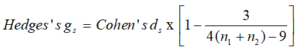
For Cohen’s ds and Hedges’s gs the extents are denoted as 0.01 > very small effect; 0.20 > small effect; 0.50 > medium effect; 0.80 > large effect; 1.20 > very large effect; based on the standards from Cohen and Sawilowsky [44, 45].
Results
ApEn for controls and COPD subjects with values for tolerance, r (0.1→0.5 in intervals of 0.1) and embedding dimension, M (1→5 in intervals of 1) are illustrated (Table 1). At M = 1 and M = 2, all of the values for r are appropriate as COPD has lesser chaotic response than the control and so negative effect sizes throughout. Effect size values for these parameters are between -0.40 and -1.13 (small to large effect sizes). These are significant and physiologically suitable. At that point, as M increases additional values for r become inappropriate exhibiting positive effect sizes. For M = 3 and r = 0.1, this is non-valid and with M = 4 and M = 5 the tolerances of r = 0.1 and r = 0.2 are likewise invalid and so dismissed. For M = 3 and M = 4 when the values are physiologically valid at different levels of tolerance the effect sizes are between -0.53 and -0.83 (medium to large effect sizes). To conclude, at M = 5 for tolerances, r of r = 0.3 to r = 0.5, the effect sizes range from -0.34 to -0.99 (small to large effect sizes).
We now inspect zones of greatest significance by their effect sizes in finer detail (Figure 1 and 2) (Table 2). From table 1, the greatest significance was achieved at M = 2 and r = 0.1. So, we assess this zone of values more intensively. Once more, we fix values for M and r. There are values for tolerance, r (0.01→0.25 in intervals of 0.01) and embedding dimension, M (1→5 in intervals of 1). For the combinations of M and r we determine that the optimal embedding dimension, M = 2 attains greatest significance when tolerance, r = 0.1. This then corresponds to an effect size of -1.13 for Cohen’s ds (large effect size) and -1.10 for Hedges’s gs (large effect size). These are the highest values of statistical significance by effect sizes attained for any of the combinations offered (Figure 2 and Table 2). They are unchanged from the optimal values in table 1.
| M | r | Approximate entropy (n = 19) | Effect sizes (ES) |
| Mean control | ± SD control | Mean COPD | ± SD COPD | Cohen’s ds | Hedges’s gs |
| 1 | 0.1 | 1.9809 | 0.2087 | 1.8642 | 0.3494 | -0.4056 | -0.3971 |
| 1 | 0.2 | 1.4038 | 0.2281 | 1.2954 | 0.3409 | -0.3738 | -0.3660 |
| 1 | 0.3 | 1.0755 | 0.2123 | 0.9571 | 0.3181 | -0.4377 | -0.4285 |
| 1 | 0.4 | 0.8400 | 0.1867 | 0.7543 | 0.2911 | -0.3506 | -0.3433 |
| 1 | 0.5 | 0.6900 | 0.1657 | 0.6007 | 0.2538 | -0.4165 | -0.4077 |
| 2 | 0.1 | 1.4006 | 0.0613 | 1.3100 | 0.0957 | -1.1279 | -1.1042 |
| 2 | 0.2 | 1.2506 | 0.1813 | 1.1322 | 0.2325 | -0.5677 | -0.5558 |
| 2 | 0.3 | 0.9934 | 0.1955 | 0.8686 | 0.2504 | -0.5557 | -0.5441 |
| 2 | 0.4 | 0.7854 | 0.1771 | 0.6913 | 0.2355 | -0.4514 | -0.4420 |
| 2 | 0.5 | 0.6469 | 0.1619 | 0.5496 | 0.2086 | -0.5207 | -0.5098 |
| 3 | 0.1 | 0.5399 | 0.1486 | 0.5975 | 0.2248 | 0.3022● | 0.2959● |
| 3 | 0.2 | 0.9635 | 0.0709 | 0.8899 | 0.1039 | -0.8279 | -0.8106 |
| 3 | 0.3 | 0.8753 | 0.1347 | 0.7657 | 0.1864 | -0.6734 | -0.6593 |
| 3 | 0.4 | 0.7217 | 0.1479 | 0.6275 | 0.1965 | -0.5415 | -0.5301 |
| 3 | 0.5 | 0.6029 | 0.1453 | 0.5053 | 0.1821 | -0.5925 | -0.5801 |
| 4 | 0.1 | 0.1275 | 0.0718 | 0.2069 | 0.1608 | 0.6375● | 0.6241● |
| 4 | 0.2 | 0.5979 | 0.1426 | 0.6068 | 0.1364 | 0.0640● | 0.0626● |
| 4 | 0.3 | 0.7145 | 0.0464 | 0.6467 | 0.1101 | -0.8019 | -0.7851 |
| 4 | 0.4 | 0.6480 | 0.1051 | 0.5603 | 0.1437 | -0.6962 | -0.6816 |
| 4 | 0.5 | 0.5556 | 0.1206 | 0.4643 | 0.1504 | -0.6703 | -0.6562 |
| 5 | 0.1 | 0.0235 | 0.0206 | 0.0571 | 0.0609 | 0.7378● | 0.7224● |
| 5 | 0.2 | 0.3082 | 0.1425 | 0.3583 | 0.1654 | 0.3249● | 0.3181● |
| 5 | 0.3 | 0.5309 | 0.1000 | 0.4986 | 0.0845 | -0.3486 | -0.3413 |
| 5 | 0.4 | 0.5680 | 0.0624 | 0.4863 | 0.0987 | -0.9891 | -0.9683 |
| 5 | 0.5 | 0.5175 | 0.1012 | 0.4274 | 0.1262 | -0.7870 | -0.7705 |
Table 1: Approximate entropy (ApEn) for controls and COPD subjects (both n = 19). Note: There were 1000 RR-intervals for each subject. Extra parameters are tolerance, r and, embedding dimension, M. There were 25 groups of values for tolerance, r (0.1→0.5 in intervals of 0.1) and embedding dimension, M (1→5 in intervals of 1). Established are the ApEn for the mean controls and their standard deviations, mean COPD and COPD standard deviations and their effect sizes (Cohen’s ds and Hedges’s gs) for control versus COPD. Where the effect sizes are positive (●) the statistical analysis is physiologically inappropriate. Where the values are in bold, these are the optimal values (in this range of M and r) for the two effect sizes Cohen’s ds and Hedges’s gs.
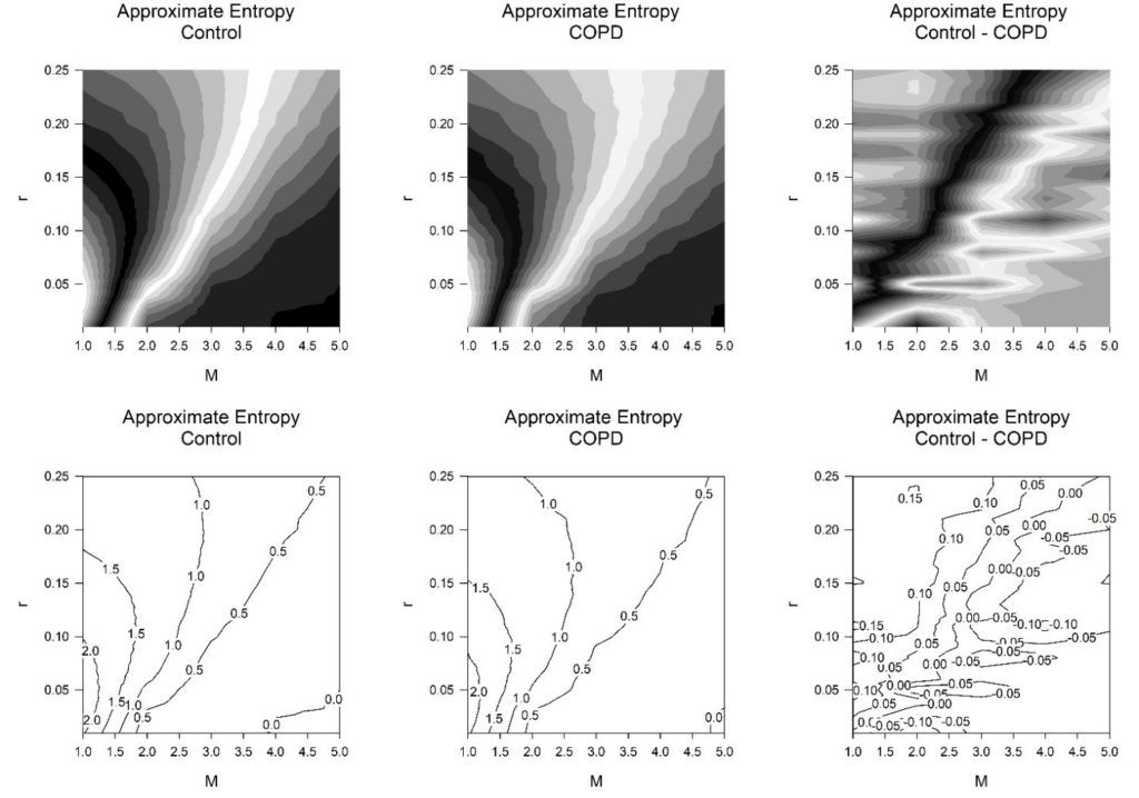
Figure 1: Contours greyscale (above) and lines (below) for the approximate entropy (ApEn) for controls (n = 19) and subjects exhibiting symptoms of COPD (n = 19). Note: In the data there were 1000 RR-intervals throughout. Values for tolerance, r (0.01→0.25 in intervals of 0.01) and, embedding dimension, M (1→5 in intervals of 1). The ApEn for the controls (left), those with COPD (middle), the difference for ApEn between the controls and those with COPD (right).
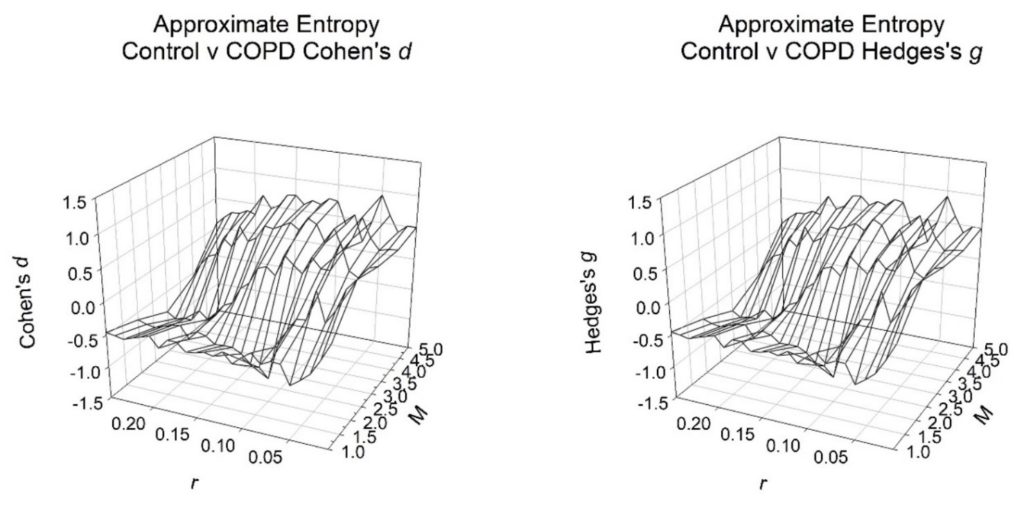
Figure 2: Effect sizes for controls versus COPD subjects (both n = 19). Note: 1000 RR-intervals were required in the calculations for each subject where, tolerance is r (0.01→0.25 in intervals of 0.01) and embedding dimension is M (1→5 in intervals of 1). The physiologically appropriate values for effect sizes are negative and so decreasing on the Cohen’s ds and Hedges’s gs axes.
| r | Effect sizes by Cohen’s ds | Effect sizes by Hedges’s gs |
| M = 1 | M = 2 | M = 3 | M = 4 | M = 5 | M = 1 | M = 2 | M = 3 | M = 4 | M = 5 |
| 0.01 | 0.0608 | 0.6127 | 0.4934 | 0.4388 | 0.5079 | 0.0595 | 0.5999 | 0.4831 | 0.4296 | 0.4973 |
| 0.02 | -0.2093 | 0.4531 | 0.4423 | 0.4242 | 0.5079 | -0.2049 | 0.4436 | 0.4330 | 0.4153 | 0.4973 |
| 0.03 | -0.4388 | 0.1128 | 0.2733 | 0.3886 | 0.3874 | -0.4296 | 0.1105 | 0.2675 | 0.3804 | 0.3793 |
| 0.04 | -0.5610 | -0.0932 | 0.3535 | 0.5558 | 0.6353 | -0.5493 | -0.0912 | 0.3461 | 0.5441 | 0.6220 |
| 0.05 | -0.6668 | 0.3584 | 0.7477 | 0.8502 | 0.9331 | -0.6528 | 0.3508 | 0.7320 | 0.8324 | 0.9135 |
| 0.06 | -0.3805 | -0.1017 | 0.3118 | 0.4976 | 0.4928 | -0.3725 | -0.0995 | 0.3052 | 0.4871 | 0.4825 |
| 0.07 | -0.3740 | -0.1163 | 0.3154 | 0.3048 | 0.1513 | -0.3661 | -0.1139 | 0.3088 | 0.2984 | 0.1481 |
| 0.08 | -0.4447 | -0.3213 | 0.4649 | 0.6151 | 0.5624 | -0.4354 | -0.3146 | 0.4552 | 0.6022 | 0.5506 |
| 0.09 | -0.3060 | -0.5901 | 0.1888 | 0.3684 | 0.3866 | -0.2995 | -0.5777 | 0.1848 | 0.3606 | 0.3785 |
| 0.10 | -0.4056 | -1.1279 | 0.3022 | 0.6375 | 0.7378 | -0.3971 | -1.1042 | 0.2959 | 0.6241 | 0.7224 |
| 0.11 | -0.5296 | -0.9781 | 0.4275 | 0.7128 | 0.7627 | -0.5185 | -0.9576 | 0.4186 | 0.6978 | 0.7467 |
| 0.12 | -0.3796 | -0.9528 | 0.0850 | 0.5090 | 0.6498 | -0.3716 | -0.9328 | 0.0832 | 0.4984 | 0.6362 |
| 0.13 | -0.4747 | -0.8210 | 0.2058 | 0.6023 | 0.6913 | -0.4647 | -0.8037 | 0.2014 | 0.5897 | 0.6768 |
| 0.14 | -0.4458 | -0.7488 | 0.1530 | 0.5294 | 0.6097 | -0.4365 | -0.7331 | 0.1498 | 0.5183 | 0.5969 |
| 0.15 | -0.4846 | -0.7479 | -0.1056 | 0.4630 | 0.7402 | -0.4745 | -0.7323 | -0.1034 | 0.4533 | 0.7247 |
| 0.16 | -0.5012 | -0.7591 | -0.2145 | 0.4852 | 0.7228 | -0.4907 | -0.7432 | -0.2100 | 0.4750 | 0.7077 |
| 0.17 | -0.3761 | -0.6554 | -0.4725 | 0.2739 | 0.5352 | -0.3682 | -0.6416 | -0.4626 | 0.2681 | 0.5239 |
| 0.18 | -0.3808 | -0.6159 | -0.5381 | 0.1918 | 0.4626 | -0.3728 | -0.6030 | -0.5268 | 0.1878 | 0.4529 |
| 0.19 | -0.5304 | -0.7528 | -0.7262 | 0.4196 | 0.6585 | -0.5193 | -0.7370 | -0.7110 | 0.4108 | 0.6447 |
| 0.20 | -0.3738 | -0.5677 | -0.8279 | 0.0640 | 0.3249 | -0.3660 | -0.5558 | -0.8106 | 0.0626 | 0.3181 |
| 0.21 | -0.4177 | -0.5999 | -0.7090 | 0.1806 | 0.3664 | -0.4089 | -0.5873 | -0.6941 | 0.1769 | 0.3587 |
| 0.22 | -0.4614 | -0.6397 | -0.8887 | -0.1110 | 0.3000 | -0.4518 | -0.6263 | -0.8701 | -0.1087 | 0.2937 |
| 0.23 | -0.5107 | -0.6871 | -0.8871 | -0.1657 | 0.2948 | -0.5000 | -0.6727 | -0.8685 | -0.1622 | 0.2886 |
| 0.24 | -0.4816 | -0.6638 | -0.9227 | -0.3305 | 0.1911 | -0.4715 | -0.6499 | -0.9034 | -0.3235 | 0.1870 |
| 0.25 | -0.4617 | -0.6158 | -0.8332 | -0.5616 | 0.0653 | -0.4520 | -0.6029 | -0.8157 | -0.5499 | 0.0639 |
Table 2: Effect sizes by Cohen’s ds and Hedges’s gs for controls versus COPD subjects (both n = 19). Exactly 1000 RR-intervals were required in the calculations for each subject. Extra parameters consist of tolerance, r and embedding dimension, M (1 →5). There were 25 values for tolerance, r (0.01→0.25, in intervals of 0.01).
Discussion
COPD has been established as a dynamical disease [2, 7, 8] which has been revealed to decrease the chaotic response and irregularities of the RR-intervals. This has previously been observed via chaotic global dimensions [2]. We then studied the responses of ApEn on the same dataset as in that chaotic global study [2] and when ApEn was systematically applied via 25 different parameters for tolerance, r (0.1→0.5 in intervals of 0.1) and embedding dimension, M (1→5 in intervals of 1); 20 out of 25 (80%) of these combinations were viable when considered physiologically. This was twice that over a similar analysis in subjects with type 1 diabetes mellitus (DM1) [28]. The COPD results signify that ApEn is capable of identifying the reduction in chaotic response and the best combination of r and M for this was 0.1 and 2, respectively.
Chaos and other irregularities typically decrease in pathological states, as observed in this study in individuals with COPD. The amount of chaotic response through ApEn has several advantages. Firstly, it can be successfully applied to short time-series (RR < 50), and secondly, it can accurately respond notwithstanding substantial levels of signal noise. Despite this, its main drawback is the selection of optimum parameters for tolerance, r and embedding dimension, M. In this study, at the outset, we applied 25 different combinations of r and M (Table 1). Later, these were studied in finer detail (Table 2). Since COPD is a pathological dynamical disease which lessens the chaotic response of HRV; those combinations of r and M which increase their responses for COPD were disregarded and they are physiologically inappropriate. These achieve positive effect sizes for Cohen’s ds and Hedges’s gs. 5 out of 25 (20%) of these permutations provided a higher value for the control than for the COPD subjects, so unsuitable. Inspecting the results (Table 1), we can observe that the optimum combination of M is 2 and r is 0.1. When we consider the values more closely regarding the tolerance, r and embedding dimension, M levels the optimal combination of r and M for this is again 0.1 and 2, respectively (Table 2 and Figure 2). This, once more calculates an effect size of -1.13 for Cohen’s ds, and -1.10 for Hedges’s gs.
Thus, in this study, ApEn has been revealed to be a significant mathematical marker if the embedding dimension, M and tolerance, r are chosen such that the differences are maximized as measured by Cohen’s ds, and Hedges’s gs. There is at present no procedure or algorithm to systematically designate these values. Therefore, ApEn can be viewed as an erratic mathematical marker which can only be applied when the M and r are optimally selected by trial and error.
Typically, when assessing HRV in studies using ApEn the fixed values are often set at M = 2 and r = 0.2 where this indicates 20% of the standard deviation of the time series [30]. Therefore, if we were enforcing ApEn in clinics or hospital units it would be too slow to calculate all the possible values of ApEn as in this study. It would necessitate implementation of multiple calculations each time to attain the specific value to evaluate a healthy or pathological condition. The optimum values here for COPD do not differ markedly to those in DM1 in the similar study [28], but the values which are physiologically accurate are more numerous in COPD. In light of these two studies on ApEn, with DM1 optimal r = 0.08 and M = 2 [28] and COPD r = 0.1 and M = 2, it is useful to re-evaluate if setting M = 2 and r = 0.2 for all datasets is appropriate. A more sophisticated approach is likely required.
Despite the advantages of ApEn, such as performing well on short time-series (RR < 50), even in the presence of signal noise; in this study ApEn has been established to be a relatively unpredictable mathematical marker. We encourage the use of other techniques, such as the chaotic global procedures [2, 13] and Katz fractal dimension [47, 48], for assessing pathological states. The Katz fractal dimension metric necessitates cubic spline interpolation [46, 47] therefore is also time expensive in circumstances where again processing speed is important. Chaotic globals are algorithmically simpler, perform well on relatively short time-series (RR > 256) [48], even with signal noise, discriminate between the groups better and need less computational time when the determination of optimal M and r is accounted for. This is imperative in situations where slow mathematical responses to physiological variables are unsuitable.
Conclusion
The ApEn was able to identify the reduction in chaotic response in COPD. The optimal combination of r and M for this were 0.1 and 2, respectively. Despite this, the ApEn has been established as an unpredictable mathematical marker requiring bespoke parameters if to be applied successfully and the use of other techniques to evaluate a healthy or pathological condition is encouraged.
Conflicts of Interest
The authors declare no conflicts of interest regarding the publication of this article.
Funding Statement
Financial support was provided by CNPq – number process: 477442/2012-9.
References
- Goldberger AL. Cardiac chaos. Science. 1989;243(4897):1419.
- Bernardo AF, Vanderlei LC, Garner DM. HRV Analysis: A clinical and diagnostic tool in chronic obstructive pulmonary disease. Int Sch Res Notices. 2014;2014:673232.
- Barreto GS, Vanderlei FM, Vanderlei LC, et al. Risk appraisal by novel chaotic globals to HRV in subjects with malnutrition. J Hum Growth Dev. 2014;24(3):243-48.
- Vanderlei FM, Vanderlei LC, Garner DM. Chaotic global parameters correlation with heart rate variability in obese children. J Hum Growth Dev. 2014;24(1):24-30.
- Ho M. The rainbow and the worm: The physics of organisms. 3rd ed. Singapore: World scientific; 2008.
- Prigogine I. Non-equilibrium statistical mechanics. New York: Interscience; 1962.
- Mackey MC, Milton JG. Dynamical diseases. Ann N Y Acad Sci. 1987;504(1):16-32.
- Chang S. Physiological rhythms, dynamical diseases and acupuncture. Chin J Physiol. 2010;53(2):77-90.
- Vanderlei LC, Silva RA, Pastre CM, et al. Comparison of the Polar S810i monitor and the ECG for the analysis of heart rate variability in the time and frequency domains. Braz J Med Biol Res. 2008;41(10):854-59.
- Rachow T, Berger S, Boettger MK, et al. Nonlinear relationship between electrodermal activity and heart rate variability in patients with acute schizophrenia. Psychophysiology. 2011;48(10):1323-332.
- Wiertel-Krawczuk A, Hirschfeld AS, Huber J, et al. Sympathetic skin response following single and combined sound and electrical stimuli in young healthy subjects. JMS. 2016;85(2):106-13.
- Baum P, Petroff D, Classen J, et al. Dysfunction of autonomic nervous system in childhood obesity: a cross-sectional study. PLoS One. 2013;8(1):e54546.
- De Souza NM, Vanderlei LC, Garner DM. Risk evaluation of diabetes mellitus by relation of chaotic globals to HRV. Complexity. 2015;20(3):84-92.
- Pincus SM. Approximate entropy as a measure of system complexity. Proc Natl Acad Sci USA. 1991;88(6):2297-301.
- Garner DM, Ling BW. Measuring and locating zones of chaos and irregularity. J Syst Sci Complex. 2014;27(3):494-506.
- Garner DМ, Alves М, Silva B, et al. Chaotic global analysis of heart rate variability following power spectral adjustments during exposure to traffic noise in healthy adult women. Russ J Cardiol. 2020;25(6):3739.
- Vanzella LM, Bernardo AF, Carvalho TD, et al. Complexity of autonomic nervous system function in individuals with COPD. J Bras Pneumol. 2018;44(1):24-30.
- Leite MR, Ramos EM, Kalva-Filho CA, et al. Correlation between heart rate variability indexes and aerobic physiological variables in patients with COPD. Respirology. 2015;20(2):273-78.
- Rossi RC, Vanderlei FM, Bernardo AF, et al. Effect of pursed-lip breathing in patients with COPD: linear and nonlinear analysis of cardiac autonomic modulation. COPD. 2014;11(1):39-45.
- Catai AM, Pastre CM, Godoy MF, et al. Heart rate variability: are you using it properly? Standardisation checklist of procedures. Braz J Phys Ther. 2020;24(2):91-102.
- Barbosa MP, Silva NT,Azevedo FM, Pastre CM, Vanderlei LC. Comparison of Polar® RS800G3™ heart rate monitor with Polar® S810i™ and electrocardiogram to obtain the series of RR intervals and analysis of heart rate variability at rest. Clin Physiol Funct Imaging. 2016;36(2):112-17.
- Takishima T, Grimby G, Graham W, et al. Flow-volume curves during quiet breathing, maximum voluntary ventilation, and forced vital capacities in patients with obstructive lung disease. Scand J Respir Dis. 1967;48(3):384-93.
- Rabe KF, Hurd S, Anzueto A, et al. Global strategy for the diagnosis, management, and prevention of chronic obstructive pulmonary disease: GOLD executive summary. Am J Respir Crit Care Med. 2007;176(6):532-55.
- American Thoracic Society. Standardization of spirometry, 1994 update. Am J Respir Crit Care Med. 1995;152(3):1107-136.
- Shannon CE. A mathematical theory of communication. SIGMOBILE Mob Comput Commun Rev. 2001;5(1):3-55.
- Pincus S. Approximate entropy (ApEn) as a complexity measure. Chaos. 1995;5(1):110-17.
- Richman JS, Lake DE, Moorman JR. Sample entropy. Methods Enzymol. 2004;384:172-84.
- Garner DM, de Souza NM, Vanderlei LCM. Unreliability of approximate entropy to locate optimal complexity in diabetes mellitus via heart rate variability. Series Endo Diab Met. 2020;2(2):32-40.
- Richman JS, Moorman JR. Physiological time-series analysis using approximate entropy and sample entropy. Am J Physiol Heart Circ Physiol. 2000;278(6):H2039-49.
- Vanderlei F, Vanderlei LC, de Abreu LC, et al. Entropic Analysis of HRV in Obese Children. Int Arch Med. 2015;8(2015)1-9.
- Tarvainen MP, Niskanen JP, Lipponen JA, et al. Kubios HRV – Heart rate variability analysis software. Comput Methods Programs Biomed. 2014;113(1):210-20.
- Cumming G. Understanding the new statistics: Effect sizes, confidence intervals and meta-analysis. 1st Ed. New York: Routledge Taylor & Francis Group; 2012.
- Grissom RJ, Kim JJ. Effect sizes for research: A broad practical approach. New Jersey: Lawrence Erlbaum Associates Publishers; 2005.
- Kazis LE, Anderson JJ, Meenan RF. Effect sizes for interpreting changes in health status. Med Care. 1989;27(3 suppl):S178-S189.
- Ryan TA, Joiner BL. Normal probability plots and tests for normality. Minitab Statistical Software: Technical Reports. The Pennsylvania State University, State College, PA. Available from MINITAB. Inc, 1976.
- Anderson TW, Darling DA. A test of goodness of fit. J Am Stat Assoc. 1954;49(268):765-69.
- Razali NM, Wah YB. Power comparisons of Shapiro-Wilk, Kolmogorov-Smirnov, Lilliefors and Anderson-Darling tests. JOSMA. 2011;2(1):21-33.
- Blanco-Topping R. The impact of Maryland all-payer model on patient satisfaction of care: A one-way analysis of variance (ANOVA). International Journal of Healthcare Management. 2020:1-8.
- McKight PE, Najab J. Kruskal-Wallis Test. The corsini encyclopedia of psychology. 2010.
- Lakens D. Calculating and reporting effect sizes to facilitate cumulative science: a practical primer for t-tests and ANOVAs. Front Psychol. 2013;4:863.
- Hedges LV, Olkin I. Statistical methods for meta-analysis. Academic Press; 2014.
- Thompson B. Effect sizes, confidence intervals, and confidence intervals for effect sizes. Psychology in the Schools. 2007;44(5):423-32.
- Kline RB. Beyond significance testing: Reforming data analysis methods in behavioral research. 1st ed. Washington, DC: American Psychological Association; 2004; p. 247-271.
- Cohen J. Statistical power analysis for the behavioral sciences. 2nd ed. New York: Routledge; 2013.
- Sawilowsky SS. New effect size rules of thumb. Journal of Modern Applied Statistical Methods. 2009;8(2):26.
- Garner DM, de Souza NM, Vanderlei LCM. Heart rate variability analysis: Higuchi and Katz’s fractal dimensions in subjects with type 1 diabetes mellitus. Rom J Diabetes Nutr Metab Dis. 2018;25(3):289-95.
- Kreyszig E. Advanced engineering mathematics. 10th ed. New York: John Wiley & Sons, INC.; 2011.
- Garner DM, Vanderlei FM, Valenti VE, et al. Non-linear regulation of cardiac autonomic modulation in obese youths: interpolation of ultra-short time series. Cardiol Young. 2019;29(9): 1196-201.
