Abstract
The use of artificial intelligence (AI) and machine learning (ML) in healthcare has seen significant growth in recent years. In this study, we explored the potential of deep learning techniques for dental teeth detection and the identification of teeth as “normal”, “implant”, “root”, “erupting”, and “missing” using X-ray images. Traditionally, dentists rely on visual-tactile methods to diagnose oral conditions. However, these methods have limitations, such as inefficiency in time spent on diagnosis, the high cost of diagnosis, and subjectivity in the diagnosis.
To address these limitations, we developed an automated algorithm that recognizes teeth structures using computer vision technology and ML methods. Our algorithm was trained on a dataset of 340 adult teeth X-ray radiographs and optimized through a series of experiments to determine the best training hyper-parameters.
The development of an AI-based clinical decision support system for dental diagnosis can increase efficiency and accuracy in clinical decision-making. Our study contributes to the field of dentistry by exploring the potential of AI and ML techniques for teeth recognition and detection. Additionally, we provided mathematical explanations of our observations to aid in the interpretation of our results.
Our optimized algorithm achieved a good precision of 78.2%. Overall, our study successfully demonstrated the potential of AI and ML in dental healthcare, specifically in teeth detection and implant identification using X-ray images.
Keywords
YOLO, YOLOv5, artificial intelligence, machine learning, object detection, teeth recognition, convolutional neural networks, dental, computer vision
Abbreviations
AI: artificial intelligence; ML: machine learning; CNNs: convolutional neural networks; mAP: mean average precision; YOLO: you only look once; FPS: frames per second; IoU: Intersection over Union; CSP: cross-stage partial; SPP: spatial pyramid pooling; GIoU: generalized IoU; DIoU: distance IoU; CIoU: complete IoU; Adam: adaptive moment algorithm; SGD: stochastic gradient descent; GD: gradient descent; RMSProp: root mean square propagation; AdamW: adaptive moment algorithm with weight decay
Introduction
The traditional healthcare system faces various challenges [1], including time-consuming diagnosis processes, limited accessibility, and inadequate storage of medical records. To address these challenges, technology has become an essential tool in modern medicine, with machine learning (ML) techniques being utilized in disease diagnosis and identification, such as Alzheimer’s disease and breast cancer [2].
Artificial intelligence (AI) has also found applications in various medical fields, including dentistry, where visual-tactile methods have traditionally been used to inspect oral conditions. However, these methods are limited in terms of time efficiency and sensitivity in detecting proximal tooth surfaces [3]. As a result, computer-aided diagnosis (CAD) has emerged as a promising solution to improve the quality and efficiency of medical image analysis [4].
In this study, we explored the potential of deep learning techniques in the field of dentistry, specifically in teeth detection and classification using X-ray images. Our approach involves training a ML model on a dataset of X-ray images to extract relevant features and classify the teeth’s condition. By leveraging deep learning algorithms, our model can detect and locate even the most challenging proximal areas, which are often limited by human vision [3].
Our study contributes to the growing body of research on the use of AI and ML in dental healthcare, demonstrating the potential of these techniques to improve diagnosis and treatment outcomes. We anticipate that our findings will pave the way for the development of more advanced clinical decision support systems, enabling more efficient and accurate dental diagnoses in the future.
Literature review
Convolutional neural networks (CNNs) have been widely used in medical image analysis to transform input images into diagnostic outputs. CNNs have proven to be successful in achieving high detection efficiency and accuracy since 1995 [5].
In dental research, teeth detection and numbering have been extensively studied. Tuzoff et al. [6] achieved good results with a sensitivity of 99.41% and precision of 99.45% using a Faster R-CNN network (VGG16-net) for teeth detection. However, manual bounding box localization limited their results, as third molars were left out. In addition, teeth numbering might be lackluster in the clinical context. Therefore, an automated system is required to identify the oral structure and state of teeth without depending on the dentist’s knowledge and experience.
Takahashi et al. [7] created a model for implant recognition using YOLOv3. An automatic implant detection system is essential to identify the nature of an implant for complicated tooth processes. The final model achieved a mean average precision (mAP) of 71%. The research also concluded on the advantage of using panoramic radiographic images as they are standardized regardless of the patient. Since the differences between implant systems are subtle, one limitation of this project is the lack of high-quality X-ray images to differentiate distinct implant systems well.
Kim et al. [8] built a tooth detection model using the Faster R-CNN network (Inception v3). While the model achieved a mAP of 76.7%, the inconsistent and unstructured shape of implant and crowns compared to normal teeth was a limitation.
Kaya et al. [9] trained a YOLOv4 model with 4545 teeth for permanent and primary teeth detection. They used YOLOv4 due to its extreme accuracy and speed. Their research centered around real-time object recognition algorithms that detected multiple objects and drew bounding boxes around each object to indicate the area of the detection. Their research achieved a mAP of 92.22%. However, one of the limitations of this research would be the fact that the X-ray images were pediatric panoramic radiographs, which rendered it challenging to build a model for permanent tooth detection and numbering. The table below provides a summary of the historical reported performance of tooth detection (Table 1).
| Research | mAP | Recall | Precision |
| Primary and permanent tooth detection (Yolov4) [9] | 92.22% | – | – |
| Tooth detection (Faster R-CNN inception v3) [8] | 76.7% | – | – |
| Tooth detection (VGG-16 CNN) [6] | – | 99.41% | 99.45% |
| Implant detection (Yolov3) [7] | 71% | – | – |
Table 1: Historical tooth detection model performance results.
While teeth numbering has been successful in many research projects, recognizing the type of teeth within the oral structure is also very important. For instance, recognizing the implant system is critical when a patient changes their doctor and clinic, as shown in Takahashi et al. [7] research. Therefore, an automated AI system that identifies the type and state of teeth can aid in the transfer of responsibility from clinic to clinic.
Objective
This study aims to address the limitations and future prospects of teeth detection models using X-ray radiographs by focusing on two key areas: (1) the ability to identify multiple types of teeth, including implants, and (2) the use of adult permanent teeth X-ray radiographs as datasets. While previous studies have reported good performance of teeth detection models using different metrics, little attention has been given to the underlying mathematics and structure of these models. Therefore, in addition to developing a teeth recognition model with panoramic radiographs that can differentiate between different types of teeth in the oral system, this project also investigates the mathematical and structural components of state-of-the-art models such as YOLOv4 and YOLOv3. By providing insights into the mathematical and structural aspects of robust networks, this project aims to contribute to the development of more effective and efficient teeth detection models.
Introduction to YOLO
You only look once (YOLO) is an object detection algorithm that uses CNNs to simultaneously classify and localize objects in an image. It is a one-stage detection algorithm, which means that it requires only a single forward propagation to make predictions. This is likely the reason for YOLO to be faster than other counterparts, such as Resnet and Mobilnet. Further, YOLO is faster than two-stage detectors, such as Faster R-CNN and Mask R-CNN.
One of the advantages of YOLO is its speed, which makes it well-suited for real-time object detection. In fact, in the Redmon et al. [10] study, YOLO outperformed other models in terms of real-time object detection with much fewer background errors (Table 2).
| Models | FPS | Error percentage |
| YOLO | 45 | 4.75% |
| Faster R-CNN | 0.5 | 13.6% |
Table 2: YOLO vs. Faster R-CNN [10].
The higher the frames per second (FPS) for YOLO, the faster it can process the input image and generate the desired output [11]. This is particularly important in the context of teeth detection and diagnosis, where good real-time object detection can increase efficiency.
To make predictions, YOLO divides the input image into an S x S grid and makes predictions for each grid cell. For each cell, the model predicts the probability of an object being present, as well as the bounding box coordinates for the object. The bounding box coordinates are normalized relative to the dimensions of the grid cell, which allows YOLO to predict objects of different sizes and aspect ratios. During training, YOLO minimizes a loss function that penalizes incorrect predictions and encourages the model to make accurate predictions.
Finally, YOLO removes duplicate and low-confidence bounding boxes to return the final object detections. This process is achieved through non-maximum suppression, which involves comparing the predicted object scores and the Intersection over Union (IoU) of the bounding boxes. The details of the YOLO architecture will be discussed in the methodology section of this report.
YOLOv5 [12] is the latest addition to the YOLO series of object detection algorithms. It was proposed by Ultralytics in May 2020 and is characterized as fast, accurate, and lightweight compared to its predecessors [13]. YOLOv5 introduces several new and unique features, including:
- Auto-learning bounding box anchors – These anchors are now smarter, allowing them to adapt to custom datasets and draw the best anchor boxes.
- New loss function for training – The CIoU loss function is used to improve accuracy and precision during training [14].
- Mosaic augmentation in YOLOv5 – This technique aids the model in learning when objects are small and improves its ability to detect them [15].
The YOLOv5 architecture can be divided into three components: backbone, neck, and head. The figure below displays a brief architecture of YOLOv5 (Figure 1).
 Figure 1: A brief architecture of YOLOv5.
The backbone is made up of cross-stage partial (CSP) layers, which extract features from the input image and generate feature maps [16]. The first layer extract features at a larger scale, while subsequent layers extract features at smaller scales. The spatial pyramid pooling (SPP) layer at the end of the backbone removes the requirement for a fixed input image size and can extract feature maps of varying sizes.
The neck is responsible for feature fusion, combining the features extracted by the CSP layers to form a unified representation of the input image. The neck comprises concatenate functions that ensure the extracted features are well collected and in the correct spatial structure before passing them to the head layer for prediction.
The head layer is in charge of prediction and consists of several convolutional layers that generate feature maps. These feature maps are processed by further convolutional layers until the final layer, where an activation function is applied to generate an output. The output contains information about the bounding box position and size, as well as the class number of the detected object.
Overall, YOLOv5 represents a significant improvement over previous YOLO models, with faster processing times and improved accuracy and precision in object detection tasks.
Methodology
The overview of our methodology is shown in the figure below (Figure 2). The subsequent subsections will follow the same flow as well.
 Figure 2: Overview of modeling process.
Datasets
Raw datasets
The raw dataset used in this study was sourced from the Tufts Dental Database [17], an online repository of radiographs created by the Panetta Visualization, Sensing, and Simulation Research Laboratory. The dataset consists of 1000 X-ray radiographs with a resolution of 1515 × 840 pixels. The radiographs were selected to support the application of AI in dental healthcare. However, the labels in the dataset are inconsistent and require processing before being used in training a model.
- Image annotation & labeling
To ensure the accuracy and consistency of our dataset, we engaged a team of dentists from the National University of Singapore [18] to assist in the annotation of the teeth in the radiographs. The dentists’ diagnoses were used as the ground truth labels, against which the model predictions were compared. After thorough discussions, we agreed on a set of five multi-class labels for each tooth: normal, missing, root, erupting, and implant, as shown in the figure below (Figure 3).

Figure 3: Classes of teeth.
Since the radiographs were unlabeled, we manually labeled 340 images using the python LabelImg package, which allowed us to draw bounding boxes around each tooth for accurate annotation. This process ensured that our dataset was labeled with precision and consistency, enabling our model to learn from high-quality data.
In order to improve the quality of the radiographs for training, we applied pre-processing techniques. The original images were too dark, with the tooth section occupying only a small portion in the middle. To address this, we used the cv2 package to crop the images and focus on the oral portion of the mouth. We also amplified the contrast of the images to increase the differences in grayscale variations for the X-ray images. The resulting images were cropped to 1200 × 600 pixels, which reduced the amount of background and helped to focus on the oral region (Figure 4).
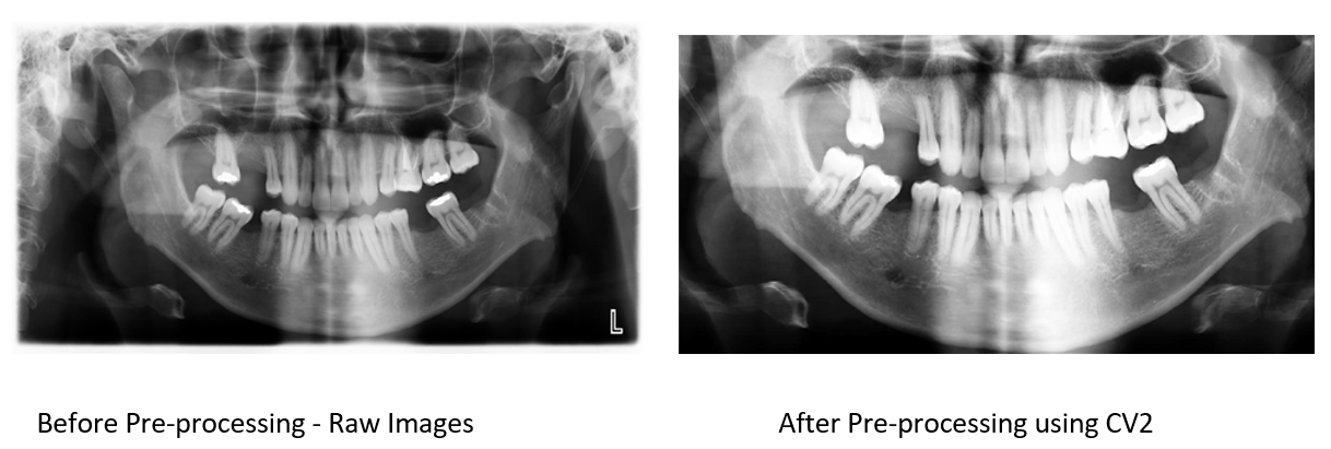
Figure 4: Pre-processing of the teeth.
Once the pre-processing was complete, we used YOLOv5’s dataloader to perform further image augmentations. The images were scaled to 640 × 640 pixels and underwent color space augmentation to improve the robustness of the model to different lighting conditions. We also applied mosaic augmentation, which helped the model to learn when objects are small and close together. Overall, these pre-processing and augmentation techniques helped to improve the accuracy and robustness of our model.
In this paper, the dataset was split into three groups: training, validation, and test. The training set was used for the computer to learn and optimize the model parameters. The validation set was used to evaluate the model during training and to calculate the evaluation metrics, such as precision, recall, and mAP, at every epoch. The test set was used to evaluate the final model after training was complete.
To ensure the dataset was well-balanced, we randomly split the train-validation-test datasets in a ratio of approximately 70-10-20. However, there was class imbalance in the distribution of the labels for each tooth, with the majority of the class labels being “normal” and “missing”. To address this issue, we ensured that the distribution of labels in our training and test sets were similar to the total distribution of the dataset, as shown in the figure below (Figure 5), by matching the blue, yellow, and green bars. This approach helped to ensure that our model was trained and tested on a balanced dataset and accurately detected all classes of teeth.
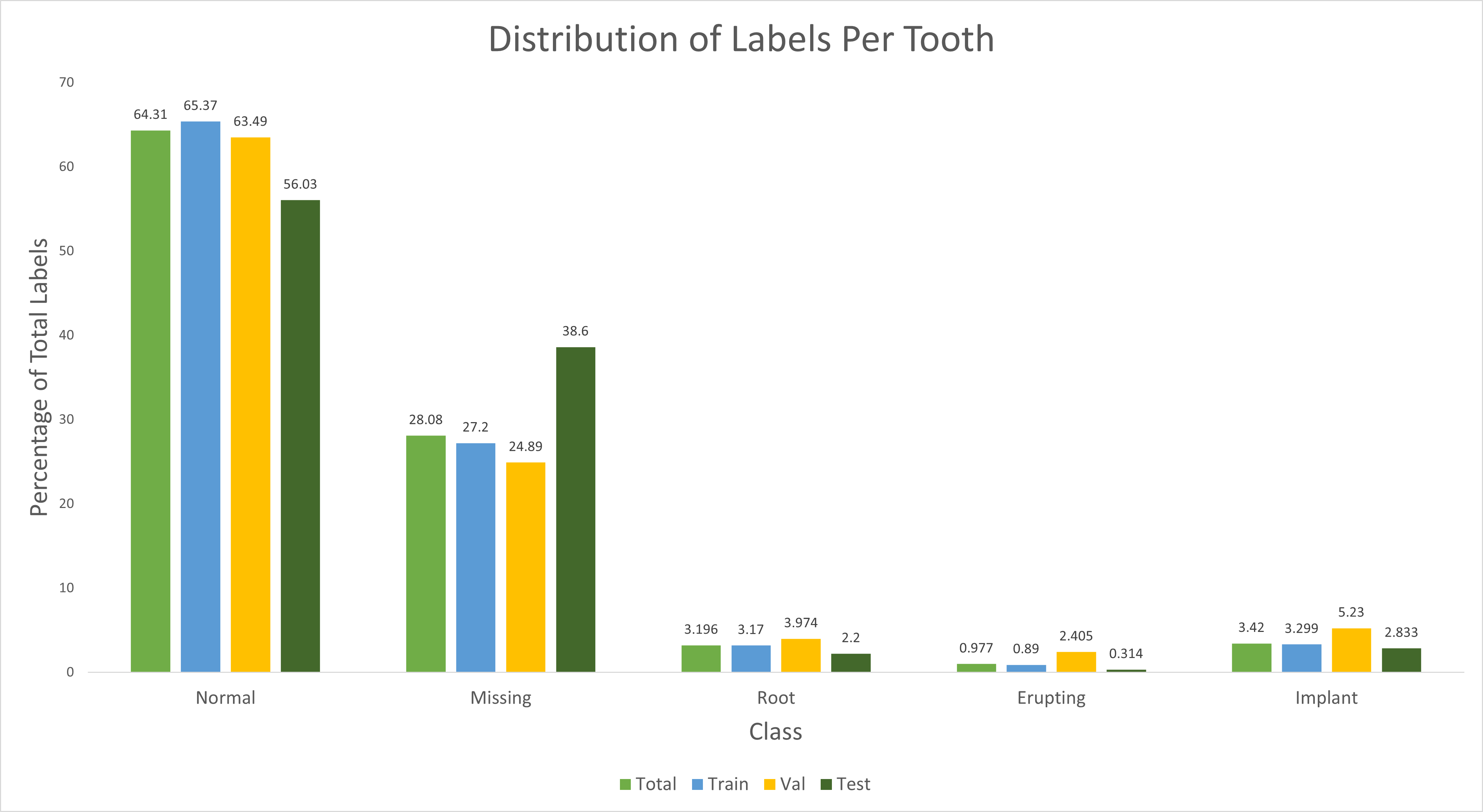
Figure 5: The proportion of labels in percentage.
Model evaluation
Various metrics were used to evaluate the performance of the model, which was designed to classify teeth into one of five categories: normal, missing, root, erupting, and implant. An additional “background” class was also included to account for unlabeled objects. There is a possibility where a certain object is not recognised as any of the five classes, and no bounding box is drawn, hence not labeled at all (background). It is important to account for such cases as it influences the precision of the model as well. Precision, recall, F1-score, and mAP were used to assess the model’s performance. The table below displays the confusion matrix and helps to explain the definitions for true positives, true negatives, false positives, and false negatives classifications for erupting teeth (Table 3).
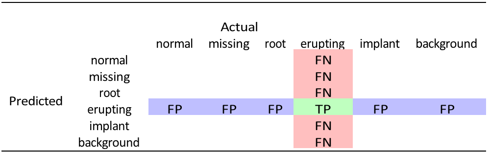 Table 3: Confusion matrix.
- True positives (TP) – Erupting class predicted correctly (green).
- False negatives (FN) – Erupting class predicted to be another class (red).
- False positives (FP) – Non-erupting class, predicted to be erupting (blue).
- True negatives (TN) – Non-erupting class, predicted correctly (white).
This study uses precision, recall, mAP, and F1-score with the specific formula as follows:
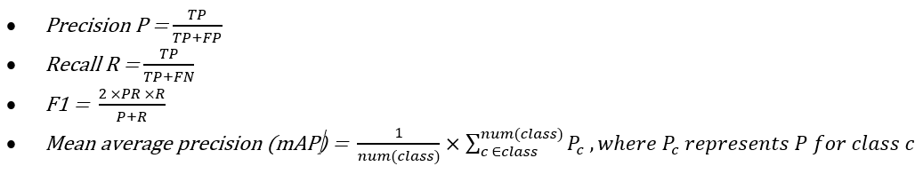
where precision measures the accuracy of the model’s positive predictions, while recall measures the proportion of actual positives that are correctly identified. The F1-score is a combination of precision and recall and takes into account the trade-off between the false positives and false negatives. mAP is an important metric for multi-class classification models, as it calculates the average precision across all classes, taking into account both false positives and false negatives. The F1-confidence curve was used to examine the relationship between the F1-score and confidence. A higher score for each metric indicates better model performance. The closer to one the score, the better the model. This study also addressed class imbalance in the dataset to ensure that the distribution of labels in the training and test sets was similar to that of the total distribution.
Model optimization
To optimize the model, a series of experiments were conducted with different parameters and settings to uncover how they affected the model’s performance. Specifically, we varied the learning rate, batch size, and number of epochs to determine the optimal combination for our model. To ensure the model’s stability and prevent overfitting, we implemented early stopping, which stops the training process when the validation loss stops improving. The hyperparameters and settings that produced the best results were selected as the final configuration for our model.
The first experiment aims to investigate the impact of sample size on model training. Two datasets containing 100 and 340 images, respectively, will be compared, and it is hypothesized that the larger dataset will result in better performance. It is crucial to assess the effect of sample size on model performance since it can impact the model’s ability to generalize to unseen data. Additionally, this experiment will explore how altering other parameters can mitigate the limitations of a small sample size.
- Intersection over Union (IoU) loss function
In the next experiment, we will examine how the IoU loss function affects model performance. In object detection, there are three types of losses: bounding box regression loss, classification loss, and objectness loss. In this paper, we will focus on the bounding box regression loss and explore the mathematical principles behind this function to gain a better understanding of how it impacts the overall performance of the model.
Bounding box regression loss (box loss) is the loss function that gives the error between the predicted and actual bounding box. Traditionally, it is calculated using IoU, where box loss LIoU = 1 − IoU, IoU (A, B) = (A ∩ B) / (A ∪ B), where A (red) is the actual bounding box and B (blue) is the predicted bounding box. Thus, IoU captures the detection effect of the predicted bounding box. Yet, it has certain disadvantages [19].
- In the case where the predicted bounding box and actual bounding box do not intersect, IoU (A, B) = 0. The error between the two boxes cannot be modeled using IoU, and the loss function is no longer capable of reducing the error (Figure 6A).
- In the case where the predicted bounding box lies within the actual bounding box, IoU is not capable of accounting for the exact position of the bounding box (Figure 6B).
- In the case where the aspect ratio of the predicted bounding box is different, yet IoU is the same. The loss is not able to account for the different aspect ratio of the bounding box (Figure 6C).
 Figure 6: Disadvantages of IoU.
Therefore, given the limitations of traditional IoU, there are several new loss functions to overcome such disadvantages – generalized IoU (GIoU), distance IoU (DIoU), and complete IoU (CIoU), where CIoU is one of the unique features of Yolov5.
a. Generalized IoU (GIoU)

where C is the smallest box containing A and B. GIoU solves the problem when A and B are disjoint, where the predicted bounding box will inch towards the actual box [20]. This way, GIoU could better reflect the level of overlap between the two bounding boxes [21]. However, GIoU loss may not converge well while using state-of-the-art detection algorithms, yielding inaccurate detection.
b. Distance IoU (DIoU)
 Where
Where
bA = centroid of actual bounding box
bB = centroid of actual predicted box
c = square of diagonal length of C
p = Euclidean distance between bA and bB
DIoU can directly minimize the distance between A and B, which allows the LossDIoU to converge much faster than LossGIoU [18]. Yet, DIoU did not take into account the difference in aspect ratio.
c. Complete IoU (CIoU)

where α = weight parameter

ν = measure of consistency of aspect ratio of actual and predicted bounding box
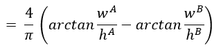
wi, hi = width and height of bounding boxes i, i ε A, B as shown in the figure (Figure 7).
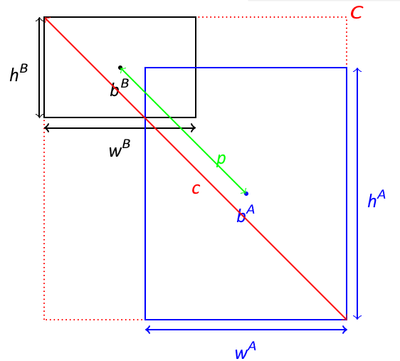 Figure 7: CIoU diagram.
Based on DIoU, CIoU accounts for the consistency of aspect ratio using ν. It is also able to converge loss much faster than GIoU. In general, since CIoU takes into account 3 factors: overlapping area, centroids, and aspect ratio, we believe that using CIoU thus leads to better performance and results.
The next set of experiments involves fine-tuning our model by adjusting hyperparameters. Since YOLOv5 utilizes neural networks, there are various parameters, such as weights, that impact the flow of information from the input to the final output. These weights play a crucial role in determining the accuracy and precision of the model in classifying the target bounding box to the correct class. In order to optimize these weights, we will fine-tune three specific hyperparameters and test different combinations to determine which yields the best results.
a. Learning rate
Learning rate is a hyperparameter that has a pivotal role in optimizing the model. It controls the magnitude at which the parameters are updated after each iteration in order to minimize the loss function of the model at every iteration. In order for our optimizer to minimize loss function well, the learning rate must be of the appropriate value. When the learning rate is too small, the model might take very long to converge. If the learning rate is too high, the model may overshoot the optimal solution and end up oscillating around it without converging.
The default learning rate is 0.01 for YOLOv5. According to Kaya et al. [9] and Jayasinghe et al. [22], for object detection, learning rates are up to 3 decimal places. Thus, we explored learning rates of 0.0001 and 0.001 as well. We hypothesized that learning rates of 0.001 or 0.0001 may perform better than the default learning rate of 0.01 because for object detection, learning rates with up to 3 decimal places perform better.
b. Optimizers
Optimizers play a crucial role in correcting the weights and parameters of a model gradually during training to minimize the loss and errors. Although there is no established rule for choosing optimizers, previous studies have provided insights that can guide the selection process. For instance, the adaptive moment algorithm (Adam) is a popular choice that has been shown to outperform stochastic gradient descent (SGD) in many cases [23]. Therefore, we will use Adam as our primary optimizer in this study. To better understand these optimizer algorithms, we will briefly explore their mechanics that were presented in previous research [24].
(i) Stochastic gradient descent (SGD)
SGD is a variant of gradient descent (GD) that updates its parameters using randomly selected input data instead of the entire dataset. This means that at each iteration, SGD only selects a small subset of observations to compute the gradient, as shown in Algorithm 1 below, making it faster than GD. However, because SGD only uses a subset of the data, it may result in a noisy estimate of the true gradient, which can lead to fluctuations in the optimization process.

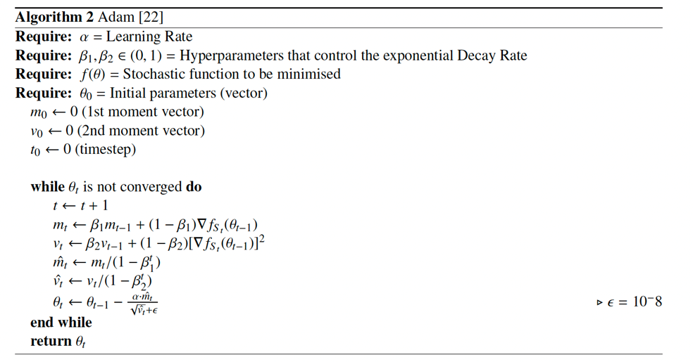
(ii) Adaptive moment algorithm (Adam)
Adam is an optimization algorithm that combines the advantages of both SGD and the root mean square propagation (RMSProp). Adam calculates the first moment (m), which is the exponentially weighted average of the gradients, and the second moment (v), which is the exponentially weighted average of the squared gradients. The algorithm then uses these values to update the parameters. As shown in Algorithm 2 below, the decay rates, β1 and β2, control how much weight is given to the previous average and the current gradient. Additionally, to overcome the initialization bias of setting m0 and v0 to 0, the algorithm normalizes mt and vt to  and
and  respectively. This prevents mt and vt from being close to 0, which can slow down the optimization process [25]. Overall, Adam is known to perform well in a variety of deep learning tasks and is often preferred over SGD [23].
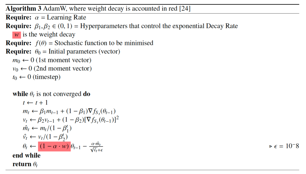
(iii) Adaptive moment algorithm with weight decay (AdamW)
The adaptive moment algorithm with weight decay (AdamW) is an extension of the Adam optimizer that incorporates weight decay regularization into the optimization process. As shown in Algorithm 3, the weight decay term is represented by the symbol ‘w’ and is applied to the weight parameters during optimization without affecting the first and second moment estimates or  . In contrast to SGD, Adam and AdamW normalize the gradient update, ∇fst, by dividing it by a running estimate of the standard deviation of the gradients. This normalization step helps to prevent the update steps from being too large or too small, which can lead to unstable convergence. Additionally, AdamW has been shown to be more robust to the choice of hyperparameters than the original Adam optimizer, making it a popular choice for deep learning practitioners.
c. Number of epochs
The number of epochs is a crucial hyperparameter that determines how many times the entire dataset is iterated during training. It is important to note that a large epoch size does not always result in better performance and can even lead to overfitting of the training data if the number of epochs is too high. Therefore, it is essential to find the optimal number of epochs for a given model. In our experiments, we tested four different numbers of epochs: 125, 150, 200, and 300. Based on our hypothesis, we expect that the optimal number of epochs will be either 150 or 200, striking a balance between allowing the model to learn and preventing overfitting. By carefully selecting the appropriate number of epochs, we can ensure the reliability of our model.
Results and Discussion
Achieving the best model with high-performance metrics requires extensive experimentation. In this section, we present our findings in the order of how the model was trained initially and how it was fine-tuned to achieve the best performance.
Sample size
First, we evaluated the impact of the sample size on model performance. We found that building a computer vision model with only 100 images is insufficient (Figure 8). The precision, recall, and mAP scores were consistently higher for the 340-image dataset than for the 100-image dataset (Figures 8A, B, and C). In terms of loss, the values were also consistently lower for the 340-image dataset (Figures 8D, E, G, and H), except for objectness loss, which was higher for the 340-image dataset (Figure 8I).
 Figure 8: The performance between sample size of 100 images vs. 340 images.
The table shows that all four metrics were higher for the 340-image dataset in the final evaluation using the validation set (Table 4). These results suggest that using more data can improve model performance.
| Evaluation | 100 images | 340 images |
| Precision | 0.793 | 0.893 |
| Recall | 0.455 | 0.773 |
| mAP | 0.479 | 0.809 |
| F1-score | 0.4 | 0.82 |
Table 4: Evaluation of different sample sizes (100 vs. 340 images).
IoU analysis
IoU – a metric used to evaluate deep learning algorithms by estimating how well a predicted mask or bounding box matches the ground truth data. The regression loss function is a key factor in the training and optimization process of object detection. The current mainstream regression loss functions are the IoU and CIoU. The GIoU gives inaccurate regression in case of extreme aspect ratios. DIoU loss uses the normalized distance between the predicted box and ground truth and converges much faster in training than IoU and GIoU losses. CIoU loss is an aggregation of the overlap area (IoU), distance (DIoU), and aspect ratio. According to the results of our IoU analysis, CIoU outperformed GIoU and DIoU in terms of mAP. This is likely due to the fact that CIoU takes into account the aspect ratio of bounding boxes during the optimization process, which can lead to more accurate object detection. The results of our evaluation metrics also support this conclusion, as CIoU achieved higher levels of precision, recall, mAP, and F1-score compared to GIoU and DIoU (Table 5). These findings support our earlier observation that CIoU can perform better than the other two IoU metrics due to its ability to incorporate all relevant factors into the loss function.
| Evaluation | CIoU | DIoU | GIoU |
| Precision | 0.893 | 0.876 | 0.851 |
| Recall | 0.773 | 0.706 | 0.739 |
| mAP | 0.809 | 0.78 | 0.785 |
| F1-score | 0.82 | 0.77 | 0.78 |
Table 5: IoU comparison.
Hyperparameters analysis
In the hyperparameter analysis, we aimed to optimize the model’s performance by experimenting with different settings. We started by gathering the model weights from the initial training and then continued training by modifying some hyperparameters and observing the performance changes.
From Figure 8, we observed that most of the lines plateau after a certain number of epochs, indicating the presence of overfitting. However, in Figure 9A, there was a spike in precision at around 125 epochs. Therefore, reducing the number of epochs to around 150 could achieve faster results without compromising performance.
 Figure 9: The performance using different epochs.
From Figures 9D, E, F, G, and H, we observed that 150 epochs (green) showed the lowest loss values. Additionally, in Figure 9B, 150 epochs resulted in the maximum recall value compared to the other epochs. Therefore, we decided to proceed with training the model for 150 epochs to achieve optimal performance.
We applied 3 learning rates: 0.01, 0.001, and 0.0001, which would be discussed alongside the optimizers. The figures below show the performance of the optimizers for the three learning rates (Figures 10, 11, and 12).
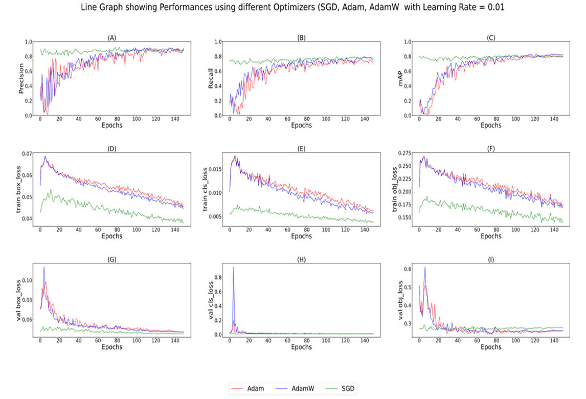 Figure 10: Performance for 150 epochs @ LR = 0.01 for different optimizers.
 Figure 11: Performance for 150 epochs @ LR = 0.001 for different optimizers.
 Figure 12: Performance for 150 epochs @ LR = 0.0001 for different optimizers.
In this study, we compared the performance of three optimizers, Adam, AdamW, and SGD, by varying the learning rate (Tables 6, 7, and 8).
 Table 6: Optimizer and learning rates comparison.
 Table 7: Optimizer and learning rates comparison.
 Table 8: Optimizer and learning rates comparison.
For a learning rate of 0.01, SGD performed the best in terms of minimum losses and maximum precision, recall, and mAP. However, for a learning rate of 0.001, Adam was found to be the best optimizer, achieving similar precision, recall, and mAP values as AdamW and SGD but with lower losses. Furthermore, Adam and AdamW showed similar performance for a learning rate of 0.0001, with AdamW having lower training losses than SGD. Based on the class-specific analysis, Adam and AdamW were found to perform better than SGD for most of the classes.
We also observed that a learning rate of 0.001 with Adam achieved the highest recall and mAP for most of the classes, which suggests that Adam is better at handling noisy and volatile gradients caused by more iterations required to converge at a smaller learning rate.
To select the final model, we considered both the general performance of the model (Table 9) and the class-specific analysis (Tables 6, 7, 8).
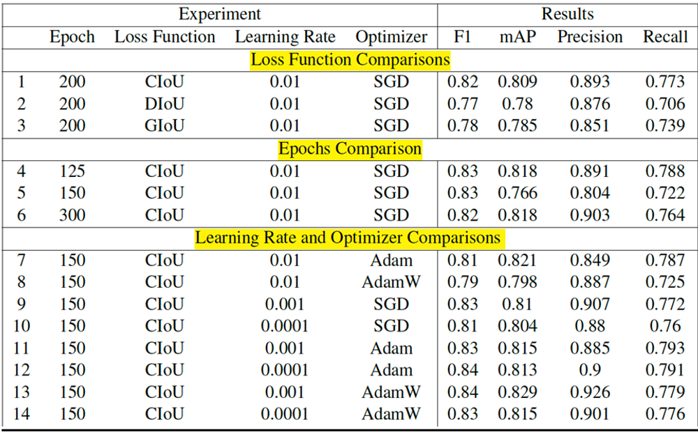 Table 9: Summary of experiments.
Based on the overall results, we chose Adam with a learning rate of 0.001 as our final optimizer for the best performance.
Conclusion
Our research work focused on the development of a teeth recognition system using the YOLOv5 object detection model. We trained and evaluated our model on a dataset of 340 fully labeled teeth images and experimented with different hyperparameters, optimizers, and learning rates to achieve the best performance. The results showed that Adam optimizer with a learning rate of 0.001 and 150 epochs performed the best in terms of precision, recall, and mAP.
Below is a summary of what was already known on the topic and what this study added to our knowledge (Table 10):
| What was already known on the topic | What this study added to our knowledge |
| Tooth detection is a crucial task in dentistry and has been tackled with various deep learning models. | This study focused on using the YOLOv5 model for tooth detection, which has not been extensively explored in dental imaging. YOLOv5 is a good computer vision technology for detecting teeth and drawing boundary boxes. |
| Optimizers play an important role in improving model performance. | This study compared the performance of three different optimizers (Adam, AdamW, and SGD) and found that their effectiveness varies depending on the learning rate and dataset. |
| Detection of teeth, counts of teeth, and number of missing teeth. | Detection of teeth and classification of teeth (normal, erupting, implant, missing, and root) is possible with YOLOv5 (2 in 1 software). |
| IoU analysis: IoU – a metric used to evaluate deep learning algorithms by estimating how well a predicted mask or bounding box matches the ground truth data. The regression loss function is a key factor in the training and optimization process of object detection. The current mainstream regression loss function is the IoU and CIoU. | CIoU achieves higher levels of precision, recall, mAP, and F1-score compared to GIoU and DIoU. |
Table 10: Summary of contributions.
Our results suggest the importance of optimizing model parameters for improving performance on object detection tasks.
In terms of limitations, for every AI project, sample size is a critical limitation, and our study is no exception. Despite creating labels from scratch, we could only gather 340 fully labeled images for experimentation. This limited sample size might have hindered our model’s ability to generalize to a broader range of scenarios. Additionally, our choice of randomly splitting datasets into a 70-10-20 ratio for training, validation, and testing may have resulted in data imbalance issues. Further research could explore other sampling methods, such as cross-validation and stratified sampling, which might help overcome these limitations. Moreover, the selection of optimizers and learning rates is a subjective and challenging process with no concrete rules. Our study examined three popular optimizers – SGD, Adam, and AdamW – but other optimizers, such as AdaGrad, RMSProp, and Nesterov, could be investigated in teeth recognition to gain new insights and achieve better results. Thus, further research could explore the efficacy of these optimizers in dental image recognition.
This project focuses only on YOLOv5, which has immense potential in real-time object detection. Future works could be done in the following areas:
- Develop a real-time teeth detector in clinical settings: You can explore the possibility of integrating the YOLOv5 model into a clinical setting and testing its effectiveness in real-time tooth detection. This could be useful in dental clinics and hospitals where patients can get instant feedback on the condition of their teeth.
- Explore the use of transfer learning: Transfer learning is a powerful technique that involves training a model on a large dataset and then fine-tuning it on a smaller dataset for a specific task. You can explore the use of transfer learning with the YOLOv5 model to improve the accuracy of tooth detection.
- Investigate the use of other deep learning models: While YOLOv5 is a powerful deep learning model, there are many other models that can be explored for tooth detection, such as Faster R-CNN (ResNet), RetinaNet, and Mask R-CNN. You can investigate these models and compare their performance with the YOLOv5 model.
- Develop a tooth segmentation model: Tooth segmentation involves separating the teeth from the rest of the image. This can be useful in applications where only the teeth need to be analyzed. You can develop a tooth segmentation model using deep learning techniques and compare its performance with the tooth detection model.
- Expand the dataset: As mentioned earlier, the limited size of the dataset is a limitation of this study. You can expand the dataset by collecting more images of teeth from different sources and with different conditions. This can improve the accuracy and generalizability of the tooth detection model.
While the most common dataset in dentistry is X-ray radiographs, it is also possible to use iPhone images. In fact, a teeth recognition model using iPhone images may bring breakthroughs in dental healthcare due to the highly ubiquitous use of the iPhone [26].
References
- Singh P, Singh N, Singh KK, et al. Diagnosing of disease using machine learning. In: Singh KK, Elhoseny M, Elngar AA. Machine Learning and the Internet of Medical Things in Healthcare. Academic Press; 2021. p. 89-111.
- Ahsan MM, Luna SA, Siddique Z. Machine-Learning-Based Disease Diagnosis: A Comprehensive Review. Healthcare (Basel). 2022;10(3):541.
- Schwendicke F, Elhennawy K, Paris S, et al. Deep learning for caries lesion detection in near-infrared light transillumination images: A pilot study. J Dent. 2020;92:103260.
- Litjens G, Kooi T, Bejnordi BE, et al. A survey on deep learning in medical image analysis. Med Image Anal. 2017;42:60-88.
- Lo SB, Lou SA, Lin JS, et al. Artificial convolution neural network techniques and applications for lung nodule detection. IEEE Trans Med Imaging. 1995;14(4):711-18.
- Tuzoff DV, Tuzova LN, Bornstein MM, et al. Tooth detection and numbering in panoramic radiographs using convolutional neural networks. Dentomaxillofac Radiol. 2019;48(4): 20180051.
- Takahashi T, Nozaki K, Gonda T, et al. Identification of dental implants using deep learning-pilot study. Int J Implant Dent. 2020;6(1):53.
- Kim C, Kim D, Jeong H, et al. Automatic Tooth Detection and Numbering Using a Combination of a CNN and Heuristic Algorithm. Applied Sciences. 2020;10(16):5624.
- Kaya E, Gunec HG, Gokyay SS, et al. Proposing a CNN Method for Primary and Permanent Tooth Detection and Enumeration on Pediatric Dental Radiographs. Journal of Clinical Pediatric Dentistry. 2022;46(4):293-98.
- Redmon J, Divvala S, Girshick R, et al. You Only Look Once: Unified, Real-Time Object Detection. 2016.
- Saxena P. Increase Frame Per Second (FPS) rate in the Custom Object Detection Step by step. 2020.
- Jocher G. ultralytics/yolov5. 2020.
- Jiang P, Ergu D, Liu F, et al. A Review of Yolo Algorithm Developments. Procedia Computer Science. 2022;199:1066-073.
- Solawetz J. What is YOLOv5? A Guide for Beginners. 2020.
- Bochkovskiy A, Wang CY, Liao HYM. YOLOv4: Optimal Speed and Accuracy of Object Detection. 2020.
- He K, Zhang X, Ren S, et al. Spatial Pyramid Pooling in Deep Convolutional Networks for Visual Recognition. 2014.
- The Tufts Dental Database.
- Vinicius Rosa; Ferreira Sabino Clarice; Deby Fajar Mardhian. Dentist from the Faculty of Dentistry, National University of Singapore.
- Wang J, Xiao H, Chen L, et al. Integrating Weighted Feature Fusion and the Spatial Attention Module with Convolutional Neural Networks for Automatic Aircraft Detection from SAR Images. Remote Sens. 2021;13(5):910.
- Zheng Z, Wang P, Liu W, et al. Distance-IoU Loss: Faster and Better Learning for Bounding Box Regression. 2019.
- Wang Z, Wu L, Li T, et al. A Smoke Detection Model Based on Improved YOLOv5. Mathematics. 2022;10(7):1190.
- Jayasinghe H, Pallepitiya N, Chandrasiri A, et al. Effectiveness of Using Radiology Images and Mask R-CNN for Stomatology. Advancements in Computing. 2022:60-65.
- Choi D, Shallue CJ, Nado Z, et al. On Empirical Comparisons of Optimizers for Deep Learning. arxiv. 2020.
- Mustapha A, Mohamed L, Ali K. Comparative study of optimization techniques in deep learning: Application in the ophthalmology field. Journal of Physics. 2021;1743(1).
- Kingma DP, Ba J. Adam: A Method for Stochastic Optimization. arxiv. 2017.
- Kumar A, Shen R, Bubeck S, et al. How to Fine-Tune Vision Models with SGD. arxiv. 2023.
