Background and Aim: The study objective was to assess chaotic global metrics in malnourished children following power spectral manipulations.
Methods: We evaluated the complexity of heart rate (HR) variability (HRV) in malnourished subjects via six power spectra (Welch, multi-taper method (MTM), Burg, covariance, Yule-Walker, and periodogram) and then, when adjusted by the MTM parameters, for further refinement. Seventy children were split equally (controls & malnourished) and the HR was monitored for 20 min; 1000 RR-intervals were attained for HRV analysis.
Results: The results stipulate that CFP1 (chaotic forward parameter) and CFP3 are the best metrics to distinguish the two groups. The most appropriate power spectra were Welch, MTM, and Yule-Walker. Results indicate that CFP3 calculated using MTM power spectra is the best combination to discriminate between the two groups. Yet, if the RR intervals are set to 400, discrete prolate spheroidal sequences (DPSS) to 3, and Thomson’s nonlinear combination to ‘adaptive’, a greater level of significance can be achieved (Cohen’s d_s = -1.57). This significantly outperforms that under default conditions (Glass’s ∆ Delta = -1.06, and Cohen’s d_s = -0.95).
Conclusion: Malnourished children have a lower response to chaotic global metrics than the control group. CFP3 with the aforementioned settings is the best combination to discriminate between these groups on the basis of RR intervals. It has the greatest significance by Cohen’s d_s. Our data suggest impaired autonomic function in malnourished children, which may have consequences for cardiovascular risks.

malnutrition, complexity, chaotic global metrics, multi-taper method, heart rate variability

HR: heart rate; HRV: heart rate variability; MTM: multi-taper method; CFP: chaotic forward parameter; DPSS: discrete prolate spheroidal sequences; ANS: autonomic nervous system; DFA: detrended fluctuation analysis; sDFA: spectral detrended fluctuation analysis; ADHD: attention deficit hyperactivity disorder; T1DM: type 1 diabetes mellitus; sMTM: spectral multi-taper method; PSD: power spectral density; DFT: discrete Fourier transform; PCA: principal component analysis

This study assesses the cardiac autonomic modulation by chaotic global analysis of heart rate variability (HRV) in malnourished children. This has been studied before [1], but here is described a more robust assessment via six power spectra and further parameter manipulations. Autonomic imbalance measured by HRV and increased cardiovascular risks has been marked in overweight children and youths [2, 3] besides the malnourished [1] and those with anorexia nervosa [4, 5].

Successive heartbeats designated as RR-intervals are consequential on the electrocardiographic PQRST motif. They have been established to oscillate in an irregular and often chaotic manner [6]. Here, we aim to evaluate the risks that malnutrition poses to the autonomic nervous system (ANS) through computations related to HRV. To complete this we executed the Shannon entropy [7] and detrended fluctuation analysis (DFA) [8] algorithms to six different power spectra to recognize which exhibited the greatest and most sensitive chaotic responses.

In 2014, Garner et al. [9] derived the spectral entropy and spectral detrended fluctuation analysis (sDFA) metrics. These were founded on the Welch power spectrum [10]. Later, their high spectral variants, hsEntropy and hsDFA were formulated and used in mathematical inverse problems by Garner et al. in 2021 [11] based on the multi-taper method (MTM) power spectrum [12]. These variants were demonstrated to be more sensitive to fluctuations in chaotic response. MTM spectra are more flexible with more parameters and have less spectral leakage.

Yet, here there are further modifications based on the covariance [13], Burg [13], Yule-Walker [14], and periodogram [15] power spectra. So, we are assessing six power spectra with the purpose of achieving results of greater significance by parametric and non-parametric statistics and three effect sizes [16] when comparing controls to malnourished children. Then, it should be possible to attain a clinical diagnosis of ANS alterations quicker and provide the required interventions sooner.

The benefit of constructing a relationship between HRV and the ANS is that it can provide a benchmark for cardiovascular risk and dynamical diseases [17, 18]. HRV is a simple, reliable, and inexpensive procedure to monitor the ANS [19, 20]. Hence, it helps to plan therapies due to early identification of health problems.

Sufficient chaotic behaviour in biomedical systems typically specifies healthy physiological status. A lessening of chaotic tendencies could be a pathophysiological marker [21]. Assessments such as these are valuable when evaluating the safety and comfort of surgical or ICU patients [21], particularly if sedated [22] or incapable of indicating distress as in sleep apnea [23] or when experiencing dyspnea [24]. We expect malnourished children to respond in a nonlinear or complex way, as occurs in subjects with attention deficit hyperactivity disorder (ADHD) [25], chronic obstructive pulmonary disease (COPD) [26], or type 1 diabetes mellitus (T1DM) [27] amongst others. The chaotic global metrics should be able to discriminate healthy from malnourished children.

Methods and materials were exactly as in the studies by Barreto et al. [1] and Garner et al. [28]. Typically, 20–25 min of RR-intervals is sufficient for chaotic global analysis [25, 29, 30]. In fact, ultra-short lengths (RR≈125) of data have been effective in obese youths [31]. The STROBE checklist [32–34] was followed throughout.

Population and sample

Seventy subjects, regardless of genders between three and five years of age were split equally: malnourished (23 girls; 3.71 ± 0.75 years; 13.02 ± 1.71 kg; 91.53 ± 5.47 cm; Z-score = -2.80 ± 0.59) or eutrophic (20 girls; 4.09 ± 0.85 years; 17.89 ± 3.04 kg; 106.83 ± 8.15 cm; Z-score = 0.191 ± 1.28). The malnourished group comprised of children less than -2 in Z-score as per the criteria for age and gender by the World Health Organization (WHO) [35]. The eutrophic group included children with Z-scores greater than or equal to -2 and less than +3, also as per the WHO criteria. Omitted from the study were obese children (Z-score greater than +3) or who had at least one of the following; taking pharmacotherapies that could affect cardiac autonomic activity, such as propranolol or atropine. Likewise, children who had infections, metabolic or cardiorespiratory system diseases that could alter cardiac autonomic control.

The subjects and parents/guardians were knowledgeable as to the study techniques and objectives and, after approving participation, they signed terms of informed consent. All techniques received consent from the ethics committee of the Institution (Process nº 275.310).

Experimental protocol

Before the experimental procedures were underway, information was logged on age, gender, mass, and height. The anthropometric measurements were assumed following the recommendations of Lohman et al. [36]. Mass was measured by a digital scale (Filizzola PL 150, Filizzola Ltda., Brazil) with a precision of 0.1 kg, with the children barefooted and dressed in light-weight clothing. Dietary and meal contents prior to the measurements were as consistent as much as possible. Height was measured via a stadiometer with a precision of 0.1 cm. The data collection was undertaken in a laboratory with the temperature maintained between 21°C and 23°C and relative humidity between 40% and 60%. Data were at all times logged between 14:00 and 17:00 to minimize circadian rhythm interferences [37, 38]. Following the initial evaluation, all techniques regarding data collection were elucidated on an individual basis and the children were told to remain at rest and not to talk during the experiment.

The heart monitor belt was positioned on the thorax, aligned with the distal third of the sternum. The Polar S810i heart rate receiver (Polar Electro, Finland) was located on their wrist. The apparatus had been validated for beat-by-beat monitoring of heart rate and the application of these datasets for HRV analysis [39]. The children were in the dorsal decubitus position on a pillow and continued at rest with natural breathing for 20 min.

After the experimental procedures, the child was discharged. The HRV behavior pattern was logged beat-by-beat during the monitoring process at a sampling rate of 1 kHz. After digital and manual filtering for the elimination of premature ectopic beats and artifacts, 1000 consecutive RR intervals were obligatory for the data analysis. Only series with > 95% sinus rhythm were included [40].

Chaotic global metrics and CFP1 to CFP7

There are three types of chaotic global metrics. They are spectral entropy, sDFA, and spectral multi-taper method (sMTM). All three were defined by Garner et al. [9]. In that case, spectral entropy and sDFA were calculated via the Welch power spectrum [14]. Later the high spectral alternatives which performed better were established and used in both forward [25, 27, 29] and mathematical inverse problems [11]. These are computed by implementing the MTM power spectrum throughout [1, 25]. These chaotic global metrics create the seven chaotic forward parameters; their non-trivial combinations. Those that are calculated using DFA respond to their chaotic sensitivities backward to the others, therefore we subtract its value from unity.

Six power spectra

Previously, the chaotic global metrics were produced via the Welch or MTM power spectra. These spectra are imposed as standard procedure for accurately estimating the chaotic globals and, their seven non-trivial permutations; CFP1 to CFP7. de Souza et al. [41] designated the application of the Welch power spectrum to achieve chaotic global metrics in subjects with T1DM.

Vanderlei et al. and Wajnsztejn et al. in similar studies described their application to youth obesity [2] and ADHD [25], respectively by applying the MTM spectra throughout. Latterly, it has been substantiated that MTM is a more adaptive and nonlinear technique, and as such it provides lesser spectral leakage. So, hypothetically should be more sensitive to chaotic and irregular responses [27].

During all these calculations the MTM power spectrum was required to compute the chaotic global metric; sMTM [9], also referred to as CFP6. sMTM (or CFP6) computes the degree of broadband noise in the system associated with increasing chaotic response.

Yet, in this study, we calculated further four spectral entropies and sDFAs. We produce an additional four using the following power spectra: covariance, Burg, Yule-Walker, and periodogram. Accordingly, including the Welch and the MTM, we attain six variants of these chaotic globals. These calculate an additional seven non-trivial permutations via these six power spectra. All three individual chaotic global metrics have a weighting of unity. Settings for these six power spectra are now defined.

When computing spectral entropy and sDFA via Welch’s method the settings are: (i) 1 Hz for sampling frequency, (ii) overlap of 50%, (iii) a Hamming window and the number of discrete Fourier transform (DFT) point to use in the power spectral density (PSD) estimate is the greater of 256 or the next power of two greater than the length of the segments, and (iv) no detrending.

Then, with MTM, the parameters are set as the following: (i) 1 Hz for sampling frequency (ii) time bandwidth for the discrete prolate spheroidal sequences (DPSS) often referred to as Slepian sequences [42] is set at 3; (iii) FFT is the larger of 256 and the next power of two greater than the length of the segment; (iv) Thomson’s ‘adaptive’ nonlinear combination method to combine individual spectral estimates is applied. DPSS is intentionally set at 3; not 5 as with Garner et al. [9, 11] as these time-series are much shorter.

The periodogram power spectral density estimate is a nonparametric estimate of a wide-sense stationary random process using a rectangular window. The number of points in the DFT is a maximum of 256 or the next power of two greater than the signal length.

Finally, for the covariance, Burg and Yule-Walker methods the order is of the autoregressive model used to produce the power spectra density estimate and is set to 16. A default DFT length of 256 is enforced.

One-way analysis of variance (ANOVA1) and Kruskal-Wallis tests

Datasets need to be normally distributed if parametric statistics are to be executed; applying the mean as an indicator of central tendency. If data normalization is unfeasible, we do not compare means. To establish the level of normality we implemented the Anderson-Darling [43], Ryan-Joiner [44], and Lilliefors [43] tests. These three tests are similar but assess normality in slightly different ways. That termed Anderson-Darling applies an empirical cumulative distribution function, whilst the Ryan-Joiner test is a correlation-based test. The Lilliefors test is beneficial when the numbers in the cohorts are low. In this study of child malnutrition, the results were mostly inconclusive. Therefore, it is impracticable to detect if the data is normal or non-normal regarding their distributions. Consequently, we computed both the one-way analysis of variance, ANOVA1 (parametric) [45] and Kruskal-Wallis (non-parametric) [46] tests of significance.

Three effect sizes

Results from ANOVA1 and Kruskal-Wallis test were often unsuccessful. They could not discriminate between the two groups when they both gave p < 0.01, (or, < 1%). Accordingly, it is suitable to compute their effect sizes [47]. Cohen’s d_s [16] is the prime subcategory of effect sizes. It refers to the standardized mean difference between two groups of independent observations for an appropriate sample [48].

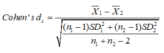
The numerator is the variation between the means of two groups of observations. The denominator is the pooled standard deviation. These differences are squared. At that point, they are summed and divided by the number of observations minus one for bias, in the estimation of the variance. To finish, the square root is applied to the denominator.

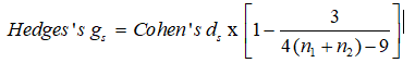
Hedges’s g_s is another effect size [49]. It is unbiased. Even so, the difference between the two is trivial, particularly with sample sizes > 20 [50].

Finally, when the standard deviations differ considerably between conditions, Glass’s ∆ delta is suitable [51]. This computes the control group’s standard deviation alone, and the experimental group is avoided.

For effects size extents they are nominated as 0.01 > very small effect; 0.20 > small effect; 0.50 > medium effect; 0.80 > large effect; 1.20 > very large effect. These are based on benchmarks by Cohen and Fritz et al. [52, 53].

Multivariate analysis by principal component analysis

Principal component analysis (PCA) [54, 55] is a statistical procedure for evaluating the complexity of high-dimensional data sets. PCA is suitable when sources of variability in the data need to be clarified or, reducing the data complexity and via this assess the data with fewer dimensions. PCA’s key objective is to characterize the data with fewer variables alongside supporting the majority of the total variance.

There are two important properties of the PCA:

1. The technique is non-parametric, so no prior information may be combined.
2. Data reduction often sustains losses in information.

There are four important procedural expectations:

1. Linearity, this identifies that the data maintains linear combinations of the variables.
2. The certainty of mean and covariance.
3. No assurance that the direction of maximum variance will contain suitable discriminative features.
4. Large variance has the key dynamics and the lowest adapts to noise.

When understanding PCA the following need consideration:

1. The higher the component loadings the more central that the variable is to that component.
2. Positive and negative loadings are recognized to be mixed.
3. The sign (+/-) of the loadings is irrelevant.
4. The rotated component matrix is vital.

RR length, Thomson’s nonlinear combinations, and DPSS

Now we assess the outcome of manipulating Thomson’s nonlinear combination settings on the MTM spectra. There are three options. The default ‘adapt’ is the adaptive frequency-dependent weights. The ‘eigen’ method weights each tapered PSD estimate by the eigenvalue (frequency concentration) of the corresponding Slepian taper. The ‘unity’ method weights each tapered PSD estimate identically [56].

Besides, in unison, we assess the outcome of altering the settings of the DPSS from 2 to 13. A DPSS equal to 1, specifies the Blackman-Tukey [57, 58] fast Fourier transform, so is excluded. It has a fixed window, so is not adaptive. Theoretically, it elicits greater spectral leakage.

DPSS affects the adaptation properties of the tapers with the purpose of diminishing spectral leakage. Whilst assessing the consequences of the Thomson’s nonlinear combinations settings and the levels of DPSS on the chaotic response, the sampling frequency is fixed at 1 Hz for the MTM and FFT is the larger of 256 and the next power of two greater than the length of the segment that is enforced. We evaluated the outcomes of DPSS (2 to 13) and Thomson’s nonlinear combinations (‘adaptive’,’eigen’, and ‘unity’). During the analysis, there are between 50 to 1000 RR-intervals. We measured both CFP1 and CFP3. These were the only permutations significant under default conditions for the Welch, MTM, and Yule-Walker power spectra. Alternative power spectra do not provide significant results. MTM is preferred as it has more constraints that can be adjusted to produce a response of the greatest significance. For CFP3 under default conditions, Yule-Walker is slightly more significant (Hedges g_s and Cohen’s d_s), but only the order can be adjusted, here it is set to 16.

ANOVA1, Kruskal-Wallis, and effect sizes

We have computed the seven versions of the three chaotic globals CFP1 to CFP7; both in controls and the malnourished children (both n = 35). Firstly, we achieved this throughout with 1000 RR intervals. The statistical results are illustrated in the six boxplots, one for each power spectrum (Figure 1).

From the table (Table 1), we noted that the combinations CFP1 and CFP3 behave equally for the Welch, MTM, and Yule-Walker power spectra. All CFP1 and CFP3 for Welch, MTM, and Yule-Walker have similar responses. They have a p < 0.01 (or, < 1%) for the ANOVA1 and Kruskal-Wallis tests of significance and, have medium to large effect sizes by all three effect size measures – Glass’s ∆ Delta, Hedges g_s, and Cohen’s d_s. They establish a decrease in chaotic response in the malnourished children group compared to the controls.

MTM (Glass’s ∆ Delta) and Yule-Walker (Hedges g_s and Cohen’s d_s) have better levels of significance when compared by their effect sizes. It is impracticable to distinguish between the two groups on the basis of the ANOVA1 and Kruskal-Wallis tests as both give p < 0.01 (or, < 1%). This is the benefit of calculating the effect sizes. They are more selective and responsive between the results.

The periodogram power spectra have a significant result for CFP3 (p < 0.01, large effect size) only. This is the best performer but cannot be manipulated to further improve as with MTM. It is, nevertheless advantageous when considering elevated levels of signal noise.

Burg and covariance give significant results for CFP2 and CFP5 (p < 0.01, medium to large effect sizes), yet the effect size values are positive and so respond in the opposite way to those options for MTM, Welch, Yule-Walker, and the periodogram designated beforehand. Those values which give positive values for the effect sizes can be disregarded. It has been established that there should be a decrease in chaotic response when comparing the controls to the malnourished children group. This was achieved in an earlier study under default conditions [1].

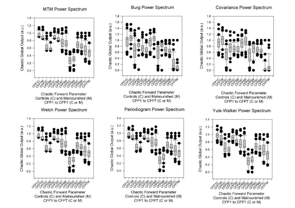
Figure 1: The boxplots of the seven combinations of chaotic forward parameters (CFP1 to CFP7) for the six power spectra density estimates (Welch, MTM, Burg, Covariance, Yule-Walker, and Periodogram) of 1000 RR intervals in control subjects (CFPx C) and those malnourished subjects (CFPx M). The point closest to zero is the minimum and the point farthest away is the maximum. The point next closest to zero is the 5^th percentile and the point next farthest away is the 95^th percentile. The boundary of the box closest to zero indicates the 25^th percentile, a line within the box marks the median (not mean), and the boundary of the box farthest from zero indicates the 75^th percentile. The difference between these points is the inter-quartile range (IQR). Whiskers (or error bars) above and below the box indicate the 90^th and 10^th percentiles respectively.

Power spectrum	CFP (1 to 7)	ANOVA1	Kruskal-Wallis	Glass’s ∆ Delta	Hedges gs	Cohen’s ds
MTM	CFP1	0.0067	0.0001	-0.7628	-0.6615	-0.6689
	CFP2	0.2835	0.3296	-0.2475	-0.2555	-0.2584
	CFP3	0.0002	<0.0001	-1.0635	-0.9399	-0.9504
	MULTI-TAPER METHODCFP4	0.5049	0.5689	-0.1623	-0.1585	-0.1602
	CFP5	0.2406	0.2219	0.2841	0.2799	0.2830
	CFP6	0.1639	0.0885	-0.3380	-0.3327	-0.3364
	CFP7	0.2238	0.2131	-0.2890	-0.2902	-0.2935
Burg	CFP1	0.1363	0.1115	0.3143	0.3564	0.3604
	BurgCFP2	0.0095	0.0057	0.5357	0.6308	0.6378
	BurgCFP3	0.0442	0.0360	-0.4542	-0.4847	-0.4901
	BurgCFP4	0.0162	0.0191	0.5302	0.5828	0.5893
	BurgCFP5	0.0001	<0.0001	0.8337	0.9653	0.9761
	BurgCFP6	0.1639	0.0885	-0.3380	-0.3327	-0.3364
	BurgCFP7	0.0128	0.0006	-0.5366	-0.6045	-0.6113
Welch	CFP1	0.0079	0.0001	-0.7436	-0.6469	-0.6541
	CFP2	0.2917	0.2799	-0.2463	-0.2512	-0.2540
	CFP3	0.0003	<0.0001	-1.0234	-0.9006	-0.9107
	CFP4	0.4735	0.5297	-0.1741	-0.1704	-0.1723
	CFP5	0.3226	0.2851	0.2378	0.2355	0.2382
	CFP6	0.1639	0.0885	-0.3380	-0.3327	-0.3364
	CFP7	0.2602	0.2263	-0.2679	-0.2684	-0.2714
Yule-Walker	CFP1	0.0056	0.0033	-0.6930	-0.6766	-0.6842
	CFP2	0.1282	0.1570	-0.3419	-0.3640	-0.3681
	CFP3	0.0001	<0.0001	-1.0303	-1.0007	-1.0119
	CFP4	0.5838	0.5609	-0.1322	-0.1301	-0.1316
	CFP5	0.1350	0.1844	0.3398	0.3576	0.3616
	CFP6	0.1639	0.0885	-0.3380	-0.3327	-0.3364
	CFP7	0.0634	0.0669	-0.4429	-0.4462	-0.4512
Periodogram	CFP1	0.0190	0.0007	-0.6568	-0.5679	-0.5743
	CFP2	0.5394	0.4773	-0.1375	-0.1458	-0.1475
	CFP3	0.0001	<0.0001	-1.1154	-0.9974	-1.0085
	CFP4	0.7830	0.8188	-0.0667	-0.0654	-0.0661
	CFP5	0.0286	0.0376	0.5042	0.5287	0.5346
	CFP6	0.1639	0.0885	-0.3380	-0.3327	-0.3364
	CFP7	0.1782	0.1844	-0.3185	-0.3216	-0.3252
Covariance	CFP1	0.1586	0.1224	0.3441	0.3370	0.3408
	CFP2	0.0080	0.0046	0.6128	0.6463	0.6535
	CFP3	0.6264	0.3752	-0.1224	-0.1156	-0.1169
	CFP4	0.2284	0.1903	0.2968	0.2873	0.2906
	CFP5	0.0080	0.0074	0.6056	0.6464	0.6537
	CFP6	0.1639	0.0885	-0.3380	-0.3327	-0.3364
	CFP7	0.2958	0.1076	0.2840	0.2491	0.2519

Table 1: Table of results for the chaotic responses (CFP1 to CFP7) derived via six power spectra (Welch, MTM, Burg, Covariance, Yule-Walker & Periodogram) for those control subjects and those children who were malnourished (both n = 35). We computed the significance (p-value) by parametric and non-parametric techniques: One way analysis of variance (ANOVA1) and Kruskal-Wallis tests of significance, respectively. We also calculated their effect sizes Glass’s ∆ Delta, Hedges g_s and Cohen’s d_s. A negative value for effect sizes indicates a decrease in response from control to malnourished children, and a positive value the opposite response. We assessed 1000 RR-intervals throughout. Level of significance is set at p < 0.01, (or < 1%) for the ANOVA1 and Kruskal-Wallis tests.

Principal component analysis

We computed the component loadings CFP1 to CFP7 for the 1000 RR-intervals of 35 malnourished children (Table 2). So, a grid of 7-by-35. The values CFP1 and CFP3 are selected as the most significant values, deduced by the power spectra; Welch, MTM, and Yule-Walker. Regrettably, the periodogram only attains significance for CFP3. For these aforementioned three power spectra CFP1 and CFP3 were the most significant throughout when established by ANOVA1, Kruskal-Wallis and Glass’s ∆ Delta, Hedges g_s and Cohen’s d_s.

Chaotic global metrics	Welch		MTM		Yule-Walker
	PC1	PC2	PC1	PC2	PC1	PC2
CFP1	0.097	-0.668	0.081	-0.674	0.020	0.601
CFP2	-0.416	-0.273	-0.420	-0.259	-0.383	0.374
CFP3	-0.136	-0.653	-0.147	-0.649	-0.161	0.559
CFP4	0.442	-0.153	0.441	-0.160	0.462	0.222
CFP5	0.453	-0.031	0.452	-0.039	0.406	0.282
CFP6	0.440	-0.166	0.439	-0.171	0.474	0.175
CFP7	-0.453	-0.037	-0.453	-0.031	-0.473	0.166

Table 2: Principal component analysis for the three appropriate power spectra (Welch, MTM, and Yule-Walker). The component loadings were calculated for CFP1 to CFP7 for the 1000 RR-intervals of 35 malnourished children. A grid of 7-by-35. Only the first two components, principal component one (PC1) and principal component two (PC2) were calculated as a consequence of steep scree plots for all three power spectral derivatives. Periodogram, Burg and Covariance are not calculated as they don’t perform appropriately on the ANOVA1, Kruskal-Wallis and Glass’s ∆ Delta, Hedges g_s and Cohen’s d_s statistical tests.

For the Welch power spectra CFP1 has the first principal component (PC1) (0.097) and the second principal component (PC2) (-0.668); but, CFP3 has the PC1 (-0.136) and the PC2 (-0.653). Only the first two components need to be considered because of the steep scree plot. The cumulative influence as a percentage is 69.4% for the PC1 and 99.9% for the cumulative total of the PC1 and PC2. The proportion of PC2 is 30.5%. CFP3 is the most robust overall combination of chaotic globals with regard to influencing the correct outcome.

For MTM power spectra CFP1 has the PC1 (0.081) and the PC2 component (-0.674); but, CFP3 has the PC1 (-0.147) and the PC2 (-0.649). Only the first two components need to be considered owing to the equally steep scree plot. The cumulative influences are comparable to the Welch power spectra above. Once more, CFP3 is the preferred overall chaotic global combination with regard to manipulating the exact outcome.

Regarding the Yule-Walker power spectrum CFP1 has the PC1 (0.020) and the PC2 (0.601); whereas, CFP3 has the PC1 (-0.161) and the PC2 (0.559). Only the first two components need to be considered as a consequence of the steep scree plot. The cumulative influence as a percentage is 57.6% for the PC1 and 96.8% for the cumulative total of the PC1 and PC2. The proportion of PC2 is 39.2%. So, CFP3 is again the best and most robust overall chaotic global combination with regard to influencing the correct outcome.

Performing PCA was unnecessary for the Burg, covariance, and periodogram power spectra results. The Burg and covariance power spectra responded incorrectly when significant achieving positive effect sizes. Or as in the case of the periodogram, only one result was significant and, thus multivariate analysis is unsuitable. PCA indicates that CFP3 is the most influential metric for Welch, Yule-Walker, but particularly the MTM power spectra. They all have steep scree plots and similar PC1 and PC2, under default conditions.

Thomson’s nonlinear combinations, DPSS, and RR length

Now we assess the consequence that the DPSS has on the significance of the results. We enforce the effect size Cohen’s d_s here, as when we calculate the ANOVA1 and Kruskal-Wallis for Welch, MTM, and Yule-Walker they all perform identically with p < 0.01 (or, < 1%). So, it is impossible to distinguish which values are optimal. The range of statistical outcomes is unable to discriminate between their results.

If we observe the results (Figure 2), we recognize that all six charts are similar. These are assessing significance by Cohen’s d_s. CFP1 and CFP3 for the three combinations of Thomson’s nonlinear combinations are comparable. The ‘adaptive’, ‘eigen’ and ‘unity’ alternatives have insignificant effects.

Nonetheless, it is imperative to know that for time-series shorter than 400 RR-intervals (RR < 400) the outcomes vary widely for the DPSS from 2 to 13. The boxplots whiskers are wide and results don’t converge. Yet, for RR-intervals greater than 400 (RR > 400) the Cohen’s d_s values are similar for all DPSS values and the whiskers of the boxplots are narrow. This indicates that DPSS is unimportant regarding the statistical outcomes with time-series greater than 400 RR-intervals. With the exception of limited results in the short time-series; the RR < 400 zone, all values for Cohen’s d_s are negative between -0.75 and -1.6. They give medium to very large effect sizes.

So, a decrease in chaotic response is achieved when comparing the controls to the malnourished children. It is similarly important to realize that the values are maximized for Cohen’s d_s at 400 RR-intervals. At RR > 400, up to RR-intervals of 1000, their significance gradually decreases. They become less negative. Therefore, it is the case that the results are most significant for short to medium length time-series, less so for longer (between 400 and 1000 RR-intervals). They do not converge statistically at lengths of RR < 400. So, it is practical to evaluate results for time-series of 400 RR-intervals. This attains optimal significance.

When we calculate the effect sizes under default conditions (Table 1) the values for Yule-Walker are greatest (Hedges g_s and Cohen’s d_s), then MTM (Glass’s ∆ Delta), and finally, Welch power spectrum. Yet, MTM has further parameters that can be adjusted to give results of potentially greater significance. It is a much more flexible power spectrum algorithmically. When we set Thomson’s nonlinear combination to ‘adaptive’, DPSS to 3, and enforce 400 RR intervals as for CFP3 (see Table 3), MTM outperforms all the other combinations (Cohen’s d_s =-1.56755, very large effect size). CFP1 performs less well on the MTM under identical conditions. Thus, CFP3 via MTM is the best mathematical marker. It outperforms the other five power spectra on Cohen’s d_s. Cohen’s d_s is the most reliable statistical test which can be applied under these circumstances.

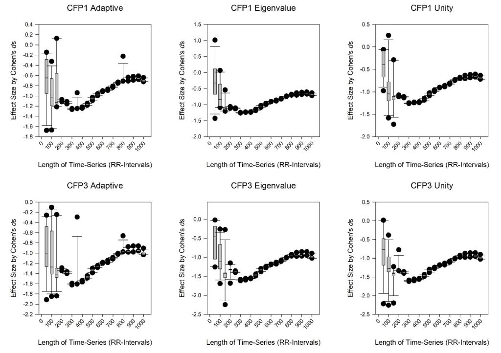
Figure 2: The boxplots of CFP1 (upper) and CFP3 (lower) for the Cohen’s d_s effect size test of significance for the controls vs. malnourished children (both n = 35). These are per DPSS values from 2 to 13 in increments of one, and for the length of time-series from 50 to 1000 RR-intervals in intervals of 50. The three Thomson’s nonlinear combinations are applied: ‘adaptive’ (upper and lower left), ‘eigen’ (upper and lower middle), and ‘unity’ (upper and lower right).

DPSS value	CFP1			CFP3
	Cohen’s ds adapt	Cohen’s ds eigen	Cohen’s ds unity	Cohen’s ds adapt	Cohen’s ds eigen	Cohen’s ds unity
2	-1.23403	-1.22723	-1.22899	-1.56128	-1.55647	-1.55763
3	-1.24385	-1.24108	-1.24142	-1.56755	-1.56545	-1.56529
4	-1.23164	-1.23128	-1.23082	-1.55432	-1.55373	-1.55299
5	-1.22131	-1.23150	-1.22919	-1.54269	-1.55501	-1.55197
6	-1.22210	-1.23206	-1.23095	-1.54281	-1.55485	-1.55320
7	-1.21711	-1.22518	-1.22390	-1.53767	-1.54702	-1.54528
8	-1.22794	-1.23059	-1.23063	-1.55068	-1.55353	-1.55334
9	-1.22783	-1.23059	-1.23061	-1.54939	-1.55307	-1.55275
10	-1.22549	-1.22786	-1.22757	-1.54662	-1.54952	-1.54881
11	-1.22924	-1.22787	-1.22771	-1.54976	-1.54872	-1.54809
12	-1.22594	-1.22575	-1.22544	-1.54682	-1.54690	-1.54626
13	-1.22935	-1.22629	-1.22622	-1.55053	-1.54757	-1.54721

Table 3: The properties of the discrete prolate spheroidal sequences (DPSS) value (2 to 13) on the effect size Cohen’s d_s when comparing chaotic globals CFP1 and CFP3 for control subjects and malnourished children (both n = 35). The remaining parameters are set as (a) sampling frequency of 1 Hz; (b) FFT is the larger of 256 and the next power of two greater than the length of the segment; (c) Thomson’s nonlinear combination methods applied (‘adapt’, ‘eigen’ and ‘unity’). 400 RR-intervals were assessed throughout.

We assessed the responses of chaotic global metrics in malnourished children related to their control group. The overall aim was to achieve an improved mathematical marker to distinguish between them. In a preceding study by Barreto et al. [1], CFP1 was indicated as the most robust function and CFP3 was the best overall statistically. Still, that study only applied the one power spectrum, MTM. So, here we attempted to verify which power spectra would perform optimally. We imposed six power spectra. Once the MTM power spectrum had been confirmed to be the best performer of the six we adjusted its properties. These data support autonomic impairment in the population evaluated.

An earlier study evaluated the impact of six power spectra in an analogous manner in subjects with T1DM [27]. Most of the conditions were identical with the exception, that with the Yule-Walker, Burg, and covariance power spectra the orders were set at 4. In this study with malnourished children and with these autoregressive power spectra we set the order to 16. When we assessed the six power spectra here, MTM was the most significant. This was similarly the case with the type 1 diabetic mellitus subjects. In this study, under default conditions, CFP3 was the best marker on the basis of five statistical tests and multivariate analysis. MTM is a useful power spectrum to impose as it can be adjusted to reduce spectral leakage. This deficit is one weakness of the other five techniques, particularly the autoregressive power spectra e.g., Burg, Yule-Walker, and covariance. A further deficit is that they are computationally expensive to compute compared to those founded on FFTs e.g., Welch, MTM, and periodogram.

To further refine the results and attempt greater significance we varied three other parameters for the MTM spectrum. These were Thomson’s nonlinear combination methods, DPSS, and the length of time-series. Here the intention was to improve the statistical outcomes. A previous study assessed this with T1DM subjects [59]. CFP3 via MTM was once more revealed to be a better marker than CFP1. No other power spectra were assessed. Then, in that study, the range of time-series was shorter at 500 to 1000 RR-intervals. Also, only ANOVA1 and Kruskal-Wallis statistical tests were executed. So, overall, it was problematic to identify the best adjustments to enhance performance. Without the effect sizes, the range of statistical outcomes is unable to differentiate straightforwardly between the two groups. In this study we computed three effect sizes; Glass’s ∆ Delta, Hedges g_s, and Cohen’s d_s. Thomson’s nonlinear combinations were set to ‘adaptive’ and DPSS to 3; as these were revealed to be the best combinations. Yet, the optimal length of the time-series was 400 RR intervals. This did not appear to be the trend in the previous study with T1DM subjects, but then, in that case, 500 RR intervals was the shortest, so cannot be confirmed.

Ultra-short time series have been assessed in obese youths [31]. In that study CFP1, CFP3 and CFP6 were all significant. But, again CFP3 performed best on Cohen’s d_s. It is difficult to discriminate with the Kruskal-Wallis test of significance alone. They all represented an increased chaotic global response in the obese youth’s group, the opposite of here with malnourished children. Despite that, the results were achieved with 125 RR-intervals, but then only that length of time-series was assessed. Performing cubic spline interpolations [60] to increase the length of time-series has repeatedly been demonstrated to be unimportant in improving the significance of the effect sizes (or, ANOVA1 and Kruskal-Wallis) between the groups. This was the case with obese youths [31] and those with T1DM [59].

The connection between malnourishment and complexity metrics is useful for ANS assessment and, indirectly, allows cardiovascular risk and dynamical disease evaluations. This is beneficial because HRV as a marker of ANS could be preferable to other neurological tests. It is easier and cheaper to administer, requiring less physician consultation time which is expensive.

CFP3 with MTM, 400 RR-intervals, Thomson’s nonlinear combination set to ‘adaptive’ and a DPSS of 3 is the best combination to discriminate between the control and malnourished children groups on the basis of RR-intervals. Malnourished children have a lower response to chaotic global metrics than the control group. Unexpectedly, if the length of the time-series is increased past 400 RR-intervals it is not always the case that the results are more significant as was the case in the default condition. In the default scenario, MTM and Yule-Walker perform similarly on the ANOVA1, Kruskal-Wallis and effect size statistical tests. Increasing the number of subjects might improve the results, but increasing the time length could be detrimental. In summary, our results indicate increased cardiovascular risk in the examined malnourished children.

Data and Matlab code enforced in the study remain confidential for commercial reasons.

The authors declare that there is no conflict of interest regarding the publication of this paper.

1. Barreto GS, Vanderlei FM, Vanderlei LCM, et al. Risk appraisal by novel chaotic globals to HRV in subjects with malnutrition. J Human Growth Development. 2014;24(3):243-48.
2. Vanderlei FM, Vanderlei LCM, Garner DM. Heart rate dynamics by novel chaotic globals to HRV in obese youths. J Human Growth Development. 2015;25(1):82-88.
3. Vanderlei FM, Vanderlei LCM, Garner DM. Chaotic global parameters correlation with heart rate variability in obese children. J Human Growth Development. 2014;24(1):24-30.
4. Koschke M, Boettger MK, Macholdt C, et al. Increased QT variability in patients with anorexia nervosa–an indicator for increased cardiac mortality? Int J Eat Disord. 2010;43(8):743-50.
5. Melanson EL, Donahoo WT, Krantz MJ, et al. Resting and ambulatory heart rate variability in chronic anorexia nervosa. Am J Cardiol. 2004;94(9):1217-220.
6. Seely AJ, Macklem PT. Complex systems and the technology of variability analysis. Crit Care. 2004;8(6):R367-84.
7. Shannon CE. A mathematical theory of communication. ACM SIGMOBILE Mobile Computing and Communications Review. 2001;5(1):3-55.
8. Bryce RM, Sprague KB. Revisiting detrended fluctuation analysis. Sci Rep. 2012;2:315.
9. Garner DM, Ling BW-K. Measuring and locating zones of chaos and irregularity. J Syst Sci Complex. 2014;27:494-506.
10. Alkan A, Kiymik MK. Comparison of AR and Welch methods in epileptic seizure detection. J Med Syst. 2006;30(6):413-19.
11. Garner DM, Ling BW-K. Measuring and locating zones of chaos and irregularity by application of high spectral chaotic global variants. Int J Bifurcation Chaos. 2021;31(15):2150236.
12. Shen C-C, Hsieh P-Y. A Flexible Speckle Reduction Strategy using Thomson’s Multitaper in High-order DMAS Beamforming. 2019 IEEE International Ultrasonics Symposium (IUS). 2019:1290-1293.
13. Subasi A. Selection of optimal AR spectral estimation method for EEG signals using Cramer-Rao bound. Comput Biol Med. 2007;37(2):183-94.
14. Alkan A, Yilmaz AS. Frequency domain analysis of power system transients using Welch and Yule–Walker AR methods. Energy Conversion Mgmt. 2007;48(7):2129-135.
15. Kiymik MK, Subasi A, Ozcalik HR. Neural networks with periodogram and autoregressive spectral analysis methods in detection of epileptic seizure. J Med Syst. 2004;28(6):511-22.
16. Cohen J. Statistical power for the behavioural sciences. Hilsdale: NY: Lawrence Erlbaum, 1988.
17. Pezard L, Nandrino JL, Renault B, et al. Depression as a dynamical disease. Biol Psychiatry. 1996;39(12):991-99.
18. Chang S. Physiological rhythms, dynamical diseases and acupuncture. Chin J Physiol. 2010;53(2)77-90.
19. Meyer M, Marconi C, Ferretti G, et al. Heart rate variability in the human transplanted heart: nonlinear dynamics and QT vs RR-QT alterations during exercise suggest a return of neurocardiac regulation in long-term recovery. Integr Physiol Behav Sci. 1996;31(4):289-305.
20. Camm AJ, Malik M, Bigger JT, et al. Heart rate variability: standards of measurement, physiological interpretation and clinical use. Task Force of the European Society of Cardiology and the North American Society of Pacing and Electrophysiology. Circulation. 1996;93(5):1043-065.
21. Seiver A, Daane S, Kim R. Regular low frequency cardiac output oscillations observed in critically ill surgical patients. Complexity. 1997;2(3):51-55.
22. Kawaguchi M, Takamatsu I, Kazama T. Rocuronium dose-dependently suppresses the spectral entropy response to tracheal intubation during propofol anaesthesia. Br J Anaesth. 2009;102(5):667-72.
23. Alvarez D, Hornero R, Marcos J, et al. Spectral analysis of electroencephalogram and oximetric signals in obstructive sleep apnea diagnosis. Annu Int Conf IEEE Eng Med Biol Soc. 2009;2009:400-403.
24. O’Donnell CR, Schwartzstein RM, Lansing RW, et al. Dyspnea affective response: comparing COPD patients with healthy volunteers and laboratory model with activities of daily living. BMC Pulm Med. 2013;13:27.
25. Wajnsztejn R, Carvalho TDD, Garner DM, et al. Heart rate variability analysis by chaotic global techniques in children with attention deficit hyperactivity disorder. Complexity. 2015;21(6):412-19.
26. Bernardo AFB, Vanderlei LCM, Garner DM. HRV analysis: A clinical and diagnostic tool in chronic obstructive pulmonary disease. Int Sch Res Notices. 2014;2014:673232.
27. Garner DM, de Souza NM, Vanderlei LCM. Risk assessment of diabetes mellitus by chaotic globals to heart rate variability via six power spectra. Romanian J Diab Nutrition Metabol Diseases. 2017;24(3):227-36.
28. Garner DM, Barreto GS, Valenti VE, et al. HRV analysis: undependability of approximate entropy at locating optimum complexity in malnourished children. Cardiol Young. 2021;32(3):425-30.
29. Garner DM, Alves M, da Silva BP, et al. Chaotic global analysis of heart rate variability following power spectral adjustments during exposure to traffic noise in healthy adult women. Russ J Cardiol. 2020;25(6):3739.
30. Fontes AM, Garner DM, de Abreu LC, et al. Global chaotic parameters of heart rate variability during mental task. Complexity. 2016;21(5):300-307.
31. Garner DM, Vanderlei FM, Valenti VE, et al. Non-linear regulation of cardiac autonomic modulation in obese youths: interpolation of ultra-short time series. Cardiol Young. 2019;29(9):1-6.
32. Knottnerus A, Tugwell P. STROBE–a checklist to strengthen the reporting of observational studies in epidemiology. J Clin Epidemiol. 2008;61(4):323.
33. Ghaferi AA, Schwartz TA, Pawlik TM. STROBE reporting guidelines for observational studies. JAMA Surg. 2021;156(6):577-78.
34. Adams AD, Benner RS, Riggs TW, et al. Use of the STROBE checklist to evaluate the reporting quality of observational research in obstetrics. Obstet Gynecol. 2018;132(2):507-12.
35. WHO, UNICEF. WHO child growth standards and the identification of severe acute malnutrition in infants and children: A joint statement by the World Health Organization and the United Nations Children’s Fund,” 2009 2009.
36. Lohman TG, Roche AF, Martorell R. Anthropometric standardization reference manual. 1988.
37. Frank G, Halberg F, Harner R, et al. Circadian periodicity, adrenal corticosteroids, and the EEG of normal man. J Psychiatr Res. 1966;4(2):73-86.
38. Kanabrocki EL, Ryan MD, Murray D, et al. Circadian variation in multiple sclerosis of oxidative stress marker of DNA damage. A potential cancer marker? Clin Ter. 2006;157(2)117-22.
39. Vanderlei LCM, Silva RA, Pastre CM, et al. Comparison of the Polar S810i monitor and the ECG for the analysis of heart rate variability in the time and frequency domains. Braz J Med Biol Res. 2008;41(10):854-59.
40. Godoy MF, Takakura IT, Correa PR. Relevância da análise do comportamento dinâmico não-linear (Teoria do Caos) como elemento prognóstico de morbidade e mortalidade em pacientes submetidos à cirurgia de revascularização miocárdica / The relevance of nonlinear dynamic analysis (Chaos Theory) to predict morbidity and mortality in patients undergoing surgical myocardial revascularization. Arq Ciênc Saúde. 2005;12(4):167-71.
41. de Souza NM, Vanderlei LCM, Garner DM. Risk evaluation of diabetes mellitus by relation of chaotic globals to HRV. Complexity. 2014;20(3):84-92.
42. Day BP, Evers A, Hack DE. Multipath suppression for continuous wave radar via slepian sequences. IEEE Transactions on Signal Processing. 2020;68:548-57.
43. Razali NM, Wah YB. Power comparisons of shapiro-wilk, kolmogorov-smirnov, lilliefors and anderson-darling tests. J Statistical Modeling Analytics. 2011;2(1):21-33.
44. Yap BW, Sim CH. Comparisons of various types of normality tests. J Statistical Comput Simulation. 2011;81(12):2141-155.
45. Hsu JC. Multiple comparisons: Theory and methods. Boca Raton, Florida: CRC Press, 1996.
46. McKight PE, Najab J. Kruskal‐wallis test. The corsini encyclopedia of psychology. 2010;1:1.
47. Kazis LE, Anderson JJ, Meenan RF. Effect sizes for interpreting changes in health status. Med Care. 1989;27(3 Suppl):S178-S189.
48. Lakens D. Calculating and reporting effect sizes to facilitate cumulative science: a practical primer for t-tests and ANOVAs. Front Psychol. 2013;26(4):863.
49. Hedges LV, Olkin I. Statistical methods for meta-analysis: Academic press, 2014.
50. Kline RB. Beyond significance testing: Retorming data analyisis methods in behavioral research. (pp. 247-271),” Washington, DC, US: American Psychological Association, 2004.
51. Becker LA. Effect size (ES). 2000;9:2007.
52. Cohen J. Statistical power analysis for the behavioral sciences: Routledge, 2013.
53. Fritz CO, Morris PE, Richler JJ. Effect size estimates: current use, calculations, and interpretation. J Exp Psychol Gen. 2012;141(1):2-18.
54. Jolliffe, I. (2005). Principal Component Analysis. In Encyclopedia of Statistics in Behavioral Science (eds B.S. Everitt and D.C. Howell).
55. Manly BF. Multivariate statistical methods: a primer. CRC Press, 2004.
56. Thomson DJ. Spectrum estimation and harmonic analysis. Proceedings of the IEEE. 1992;70(9):1055-096.
57. Bekka RE, Chikouche D. Effect of the window length on the EMG spectral estimation through the Blackman-Tukey method. Seventh International Symposium on Signal Processing and Its Applications. 2003;2:17-20.
58. Tsakiroglou E, Walden AT. From Blackman–Tukey pilot estimators to wavelet packet estimators: a modern perspective on an old spectrum estimation idea. Signal Processing. 2002;82(10):1425-441.
59. Garner DM, de Souza NM, Valenti VE, et al. Complexity of cardiac autonomic modulation in diabetes mellitus: A new technique to perceive autonomic dysfunction. Romanian J Diab Nutrition Metabol Diseases. 2019;26(3):279-91.
60. Kreyszig E. Advanced engineering mathematics: Wiley, 2011.